import pandas as pd
import numpy as np
import json

from utils.feature_engineering import *
from utils.data_cleaning import *

from sklearn.model_selection import train_test_split
from sklearn.ensemble import HistGradientBoostingClassifier 
from sklearn.metrics import accuracy_score, classification_report, f1_score


from sklearn.metrics.pairwise import cosine_similarity
from sentence_transformers import SentenceTransformer
from geopy.geocoders import Nominatim
from geopy.distance import geodesic
import time 
import warnings 


warnings.filterwarnings('ignore')

---------------------------------------------------------------------------
ModuleNotFoundError                       Traceback (most recent call last)
Cell In[1], line 5
      2 import numpy as np
      3 import json
----> 5 from utils.feature_engineering import *
      6 from utils.data_cleaning import *
      8 from sklearn.model_selection import train_test_split

ModuleNotFoundError: No module named 'utils'

Load the data

import pandas as pd 
pd.set_option('display.max_columns', None)  
df = pd.read_excel('../Dataset_2.0_Akkodis.xlsx')
df

	ID	Candidate State	Age Range	Residence	Sex	Protected category	TAG	Study area	Study Title	Years Experience	Sector	Last Role	Year of insertion	Year of Recruitment	Recruitment Request	Assumption Headquarters	Job Family Hiring	Job Title Hiring	event_type__val	event_feedback	linked_search__key	Overall	Job Description	Candidate Profile	Years Experience.1	Minimum Ral	Ral Maximum	Study Level	Study Area.1	Akkodis headquarters	Current Ral	Expected Ral	Technical Skills	Standing/Position	Comunication	Maturity	Dynamism	Mobility	English
0	71470	Hired	31 - 35 years	TURIN » Turin ~ Piedmont	Male	NaN	AUTOSAR, CAN, C, C++, MATLAB/SIMULINK, VECTOR/...	Automation/Mechatronics Engineering	Five-year degree	[1-3]	Automotive	Diagnostic/Test engineer	[2018]	[2021]	E/E Diagnostic Integration Engineer - Automotive	Milan	Engineering	Consultant	Candidate notification	NaN	NaN	NaN	The candidate, inserted within a multidiscipli...	The ideal candidate has a degree in Electronic...	[1-3]	26-28K	30-32K	Five-year degree	electronic Engineering	Modena	22-24 K	24-26 K	NaN	NaN	NaN	NaN	NaN	NaN	NaN
1	71470	Hired	31 - 35 years	TURIN » Turin ~ Piedmont	Male	NaN	AUTOSAR, CAN, C, C++, MATLAB/SIMULINK, VECTOR/...	Automation/Mechatronics Engineering	Five-year degree	[1-3]	Automotive	Diagnostic/Test engineer	[2018]	[2021]	E/E Diagnostic Integration Engineer - Automotive	Milan	Engineering	Consultant	BM interview	NaN	RS18.0145	NaN	The candidate, inserted within a multidiscipli...	The ideal candidate has a degree in Electronic...	[1-3]	26-28K	30-32K	Five-year degree	electronic Engineering	Modena	22-24 K	24-26 K	NaN	NaN	NaN	NaN	NaN	NaN	NaN
2	71470	Hired	31 - 35 years	TURIN » Turin ~ Piedmont	Male	NaN	AUTOSAR, CAN, C, C++, MATLAB/SIMULINK, VECTOR/...	Automation/Mechatronics Engineering	Five-year degree	[1-3]	Automotive	Diagnostic/Test engineer	[2018]	[2021]	E/E Diagnostic Integration Engineer - Automotive	Milan	Engineering	Consultant	Contact note	NaN	NaN	NaN	The candidate, inserted within a multidiscipli...	The ideal candidate has a degree in Electronic...	[1-3]	26-28K	30-32K	Five-year degree	electronic Engineering	Modena	22-24 K	24-26 K	NaN	NaN	NaN	NaN	NaN	NaN	NaN
3	71470	Hired	31 - 35 years	TURIN » Turin ~ Piedmont	Male	NaN	AUTOSAR, CAN, C, C++, MATLAB/SIMULINK, VECTOR/...	Automation/Mechatronics Engineering	Five-year degree	[1-3]	Automotive	Diagnostic/Test engineer	[2018]	[2021]	E/E Diagnostic Integration Engineer - Automotive	Milan	Engineering	Consultant	BM interview	OK	RS18.0114	~ 2 - Medium	The candidate, inserted within a multidiscipli...	The ideal candidate has a degree in Electronic...	[1-3]	26-28K	30-32K	Five-year degree	electronic Engineering	Modena	22-24 K	24-26 K	2.0	2.0	1.0	2.0	2.0	3.0	3.0
4	71470	Hired	31 - 35 years	TURIN » Turin ~ Piedmont	Male	NaN	AUTOSAR, CAN, C, C++, MATLAB/SIMULINK, VECTOR/...	Automation/Mechatronics Engineering	Five-year degree	[1-3]	Automotive	Diagnostic/Test engineer	[2018]	[2021]	E/E Diagnostic Integration Engineer - Automotive	Milan	Engineering	Consultant	Commercial note	NaN	NaN	NaN	The candidate, inserted within a multidiscipli...	The ideal candidate has a degree in Electronic...	[1-3]	26-28K	30-32K	Five-year degree	electronic Engineering	Modena	22-24 K	24-26 K	NaN	NaN	NaN	NaN	NaN	NaN	NaN
...	...	...	...	...	...	...	...	...	...	...	...	...	...	...	...	...	...	...	...	...	...	...	...	...	...	...	...	...	...	...	...	...	...	...	...	...	...	...	...
21372	79993	Hired	26 - 30 years	TORRE ANNUNZIATA » Naples ~ Campania	Male	NaN	X	chemical engineering	Five-year degree	[0]	Others	Graduating student	[2023]	[2023]	Junior Project Engineer (C&Q)	Pomezia	Tech Consulting & Solutions	Consultant	HR interview	OK	RS23.0793	~ 3 - High	The resource, included in a team dedicated to ...	The ideal candidate has a Master's Degree in C...	[0]	- 20K	- 20K	Five-year degree	chemical engineering	Pomezia	Not available	Not available	2.0	2.0	3.0	3.0	3.0	3.0	3.0
21373	79993	Hired	26 - 30 years	TORRE ANNUNZIATA » Naples ~ Campania	Male	NaN	X	chemical engineering	Five-year degree	[0]	Others	Graduating student	[2023]	[2023]	Junior Project Engineer (C&Q)	Pomezia	Tech Consulting & Solutions	Consultant	Candidate notification	NaN	NaN	NaN	The resource, included in a team dedicated to ...	The ideal candidate has a Master's Degree in C...	[0]	- 20K	- 20K	Five-year degree	chemical engineering	Pomezia	Not available	Not available	NaN	NaN	NaN	NaN	NaN	NaN	NaN
21374	79993	Hired	26 - 30 years	TORRE ANNUNZIATA » Naples ~ Campania	Male	NaN	X	chemical engineering	Five-year degree	[0]	Others	Graduating student	[2023]	[2023]	Junior Project Engineer (C&Q)	Pomezia	Tech Consulting & Solutions	Consultant	Candidate notification	NaN	NaN	NaN	The resource, included in a team dedicated to ...	The ideal candidate has a Master's Degree in C...	[0]	- 20K	- 20K	Five-year degree	chemical engineering	Pomezia	Not available	Not available	NaN	NaN	NaN	NaN	NaN	NaN	NaN
21375	79993	Hired	26 - 30 years	TORRE ANNUNZIATA » Naples ~ Campania	Male	NaN	X	chemical engineering	Five-year degree	[0]	Others	Graduating student	[2023]	[2023]	Junior Project Engineer (C&Q)	Pomezia	Tech Consulting & Solutions	Consultant	Technical interview	OK	RS23.0793	~ 2 - Medium	The resource, included in a team dedicated to ...	The ideal candidate has a Master's Degree in C...	[0]	20K	- 20K	Five-year degree	chemical engineering	Pomezia	Not available	Not available	2.0	2.0	2.0	2.0	2.0	3.0	3.0
21376	79993	Hired	26 - 30 years	TORRE ANNUNZIATA » Naples ~ Campania	Male	NaN	X	chemical engineering	Five-year degree	[0]	Others	Graduating student	[2023]	[2023]	NaN	NaN	NaN	NaN	NaN	NaN	NaN	NaN	NaN	NaN	NaN	NaN	NaN	NaN	NaN	NaN	Not available	Not available	NaN	NaN	NaN	NaN	NaN	NaN	NaN

21377 rows × 39 columns

Remove rows

Drop duplicates

df = df.drop_duplicates().reset_index(drop=True)

Clean the columns’ names

df = clean_dataframe_columns(df)

Create new IDs and separate different people with duplicating IDs

invariant_columns = [
    "ID",
    "Sex",
    "Job Title Hiring",
    "Study Area.1",
    "Assumption Headquarters",
    "Year of insertion",
    "Age Range",
    "Study area",
    "Study Title",
    "Years Experience",
    "Residence",
]
df = split_duplicate_ids_by_invariant_columns(df, invariant_columns)

🔵 Unique IDs before cleaning: 12263
🟢 Unique IDs after cleaning: 13372
🧮 Difference: 1109 new IDs created

Extract numer_of_searches column

df['number_of_searches'] = pd.to_numeric(
    df['linked_search__key'].str.split('.', n=1, expand=True)[1], 
    errors='coerce'
)

Remove irrelevant columns

df = df.drop(columns=['linked_search__key', 'Year of Recruitment']) 

Remove candidates in first stages

df = remove_initial_stage_candidates(df)

🗂️ Removed 7440 initial-stage only candidates.

Removal of Candidates with Inconsistent Final Outcomes

state_order = ['imported', 'first contact', 'in selection', 'qm', 'economic proposal', 'vivier', 'hired']
event_order = ['cv request', 'contact note', 'hr interview', 'bm interview', 'technical interview', 
               'qualification meeting', 'economic proposal', 'candidate notification']

grouped = df.groupby('ID', group_keys=False).apply(sort_group, state_order=state_order, event_order=event_order)

df = grouped.reset_index(drop=True)

feedbacks_to_remove = [
        'OK (other candidate)', 
        'KO (lost availability)', 
        'OK (hired)', 
        'OK (waiting for departure)', 
        'KO (opportunity closed)', 
        'KO (retired)', 
        'KO (ral)', 
        'KO (proposed renunciation)'
    ]


df = remove_not_hired_valid_candidates(df, state_order=state_order, event_order=event_order, feedbacks_to_remove=feedbacks_to_remove)

Number of unique IDs to remove: 1040
Total IDs before cleaning: 5932
Total IDs after cleaning: 4892
Total IDs removed: 1040

states_to_drop = ['vivier', 'economic proposal']

print("Before filtering:")
for c in list(set(df['Candidate State'])):
    print(f"{c}: {len(df[df['Candidate State']==c])} rows")
total_ids_before = df['ID'].nunique()

df = df[~df['Candidate State'].isin(states_to_drop)]

print("\nAfter filtering:")
for c in list(set(df['Candidate State'])):
    print(f"{c}: {len(df[df['Candidate State']==c])} rows")

total_ids_after = df['ID'].nunique()
print(f"Total IDs before cleaning: {total_ids_before}")
print(f"Total IDs after cleaning: {total_ids_after}")
print(f"Total IDs removed: {total_ids_before - total_ids_after}")

Before filtering:
qm: 399 rows
vivier: 28 rows
in selection: 3044 rows
imported: 311 rows
hired: 2143 rows
economic proposal: 46 rows
first contact: 3093 rows

After filtering:
qm: 399 rows
in selection: 3044 rows
imported: 311 rows
hired: 2143 rows
first contact: 3093 rows
Total IDs before cleaning: 4892
Total IDs after cleaning: 4870
Total IDs removed: 22

Preprocess columns

Ral Mapping

ral_mapping = {
    '- 20 K': 19000,
    '- 20K': 19000,
    '20-22 K': 21000,
    '20-22K': 21000,
    '22-24 K': 23000,
    '22-24K': 23000,
    '24-26 K': 25000,
    '24-26K': 25000,
    '26-28 K': 27000,
    '26-28K': 27000,
    '28-30 K': 29000,
    '28-30K': 29000,
    '30-32 K': 31000,
    '30-32K': 31000,
    '32-34 K': 33000,
    '32-34K': 33000,
    '34-36 K': 35000,
    '34-36K': 35000,
    '36-38 K': 37000,
    '36-38K': 37000,
    '38-40 K': 39000,
    '38-40K': 39000,
    '40-42 K': 41000,
    '40-42K': 41000,
    '42-44 K': 43000,
    '42-44K': 43000,
    '44-46 K': 45000,
    '44-46K': 45000,
    '46-48 K': 47000,
    '46-48K': 47000,
    '48-50 K': 49000,
    '48-50K': 49000,
    '+ 50 K': 55000,
    '+50K': 55000,
    '20K': 20000,
    'Not available': None,
    'Not Avail.': None,
    np.nan: None
}

ral_columns = ['Expected Ral', 'Minimum Ral', 'Ral Maximum', 'Current Ral']

for col in ral_columns:
    if col in df.columns:
        df[col] = df[col].astype(str).map(ral_mapping)
    else:
        print(f"Warning: Column '{col}' not found in the DataFrame.")

Overall mapping

print(f"The unique values of column `Overall` are {set(df['Overall'])}")

The unique values of column `Overall` are {'4 - Top', '1 - Low', nan, '~ 2 - Medium', '2 - Medium', '~ 4 - Top', '3 - High', '~ 1 - Low', '~ 3 - High'}

score_mapping = {
    '1 - Low': 1,
    '2 - Medium': 2,
    '3 - High': 3,
    '4 - Top': 4,
    '~ 1 - Low': 1,
    '~ 2 - Medium': 2,
    '~ 3 - High': 3,
    '~ 4 - Top': 4
}
df['Overall'] = df['Overall'].map(score_mapping)

Make the Protected category column boolean

df['Protected category'] = df['Protected category'].apply(lambda x: True if 'article' in str(x).lower() else False)

Remove invalid values from Job Title Hiring

df['Job Title Hiring'] = df['Job Title Hiring'].replace('???', None)

Aggregate Records

import pandas as pd
import re

def clean_text(text):
    if not isinstance(text, str) or not text.strip():
        return None
    if text.startswith('o '):
        text = text[1:].strip()
    text = re.sub(r'^[\-\•\*]+\s*', '', text.strip())

    text = re.sub(r'\s+', ' ', text)

    text = text.lower().strip()
    return text
    

for col in ['Candidate Profile','Last Role','Job Description','Candidate Profile']:
    df[col] = df[col].apply(clean_text)

def find_differences_by_id(df):
    ignore_columns = {'Job Description','event_feedback', 'event_type__val', "Overall", "Minimum Ral",'Ral Maximum', "Technical Skills", "Mobility", "English","Dynamism","Maturity","Comunication","Standing/Position"}
    id_groups = df.groupby('ID')
    counter = 0
    for id_val, group in id_groups:
        if len(group) <= 1:
            continue

        differing_cols = []
        for col in df.columns:
            if col in ignore_columns or col == 'ID':
                continue
            unique_vals = group[col].dropna().unique()
            if len(unique_vals) > 1:
                differing_cols.append((col, unique_vals))

        if differing_cols:
            if counter > 5:
                print('\n...')
                break
            else:
                counter += 1
            print(f"\nID: {id_val}")
            for col, vals in differing_cols:
                print(f"  → Column '{col}' differs: {[float(v) for v in list(vals)]}")

find_differences_by_id(df)

ID: 243
  → Column 'number_of_searches' differs: [1248.0, 1616.0]

ID: 346
  → Column 'number_of_searches' differs: [291.0, 957.0]

ID: 369
  → Column 'number_of_searches' differs: [392.0, 596.0]

ID: 1174
  → Column 'number_of_searches' differs: [1282.0, 50.0]

ID: 1242
  → Column 'number_of_searches' differs: [1102.0, 794.0, 998.0]

ID: 1301
  → Column 'number_of_searches' differs: [685.0, 531.0]

...

import numpy as np
def aggregate_group(group):
    for col in group.columns:
        if col == 'ID':
            continue  
        values = group[col].dropna().unique()
        if len(values) == 0:
            continue 
        elif len(values) == 1:
            group[col] = values[0]
        else:
            if np.issubdtype(group[col].dropna().dtype, np.number):
                avg_value = group[col].dropna().astype(float).mean()
                group[col] = avg_value
            else:
                string_values = [str(v).strip() for v in values]
                filtered_values = [v for v in string_values if v]
                combined_string = "|".join(str(v) for v in filtered_values)
                group[col] = combined_string
    return group

def aggregate_all_records(df):
    df_cleaned = df.drop(columns=['event_feedback', 'event_type__val']).drop_duplicates().reset_index(drop=True)

    grouped = df_cleaned.groupby('ID')

    groups_with_multiple = grouped.filter(lambda x: len(x) > 1)

    fixed_groups = groups_with_multiple.groupby('ID', group_keys=False).apply(aggregate_group).drop_duplicates().reset_index(drop=True)
    groups_with_single = grouped.filter(lambda x: len(x) == 1)
    final_df = pd.concat([fixed_groups, groups_with_single], ignore_index=True)

    print(f"Original number of records: {len(df['ID'])}")
    print(f"Aggregated number of records: {len(final_df['ID'])}")
    return final_df


final_df = aggregate_all_records(df)

Original number of records: 8990
Aggregated number of records: 4870

def clean_aggregated_string_column(val):
    if isinstance(val, str) and '|' in val:
        parts = val.split('|')
        filtered_parts = [p.strip() for p in parts if p.strip()]

        if not filtered_parts:
            return '' 
        elif len(filtered_parts) == 1:
            return filtered_parts[0]
        else:
            return '|'.join(filtered_parts)
    else:
        return val

def clean_aggregated_string_columns(df):
    df_cleaned = df.copy() 
    string_cols = df_cleaned.select_dtypes(include=['object', 'string']).columns

    print(f"Applying cleaning to columns: {list(string_cols)}")

    for col in string_cols:
        df_cleaned[col] = df_cleaned[col].map(clean_aggregated_string_column, na_action='ignore')

    return df_cleaned
final_df = clean_aggregated_string_columns(final_df)

Applying cleaning to columns: ['ID', 'Candidate State', 'Age Range', 'Residence', 'Sex', 'TAG', 'Study area', 'Study Title', 'Years Experience', 'Sector', 'Last Role', 'Year of insertion', 'Recruitment Request', 'Assumption Headquarters', 'Job Family Hiring', 'Job Title Hiring', 'Job Description', 'Candidate Profile', 'Years Experience.1', 'Study Level', 'Study Area.1', 'Akkodis headquarters']

Residence

with open("city_mapping.json", "r", encoding="utf-8") as f:
    city_mapping = json.load(f)
def city_transform(city):
    if city.strip().upper() in city_mapping:
        city = city_mapping[city.strip().upper()]
    else:
        city = ' '.join([c.capitalize() if c.upper() not in ['DI','IN','DEL','A'] else c.lower() for c in city.split()])
    return city

def parse_residence(residence):
    try:
        parts = residence.split('»')
    except:
        return pd.Series([None, None, None, None, False])
    city = parts[0].strip()
    if len(parts) < 2 or '~' not in parts[1]:
        italian_residence = (city.upper() == 'ITALY')  
 
        return pd.Series([city.upper(), None, None, None, italian_residence])
    subparts = parts[1].split('~')
    province = subparts[0].strip()
    region = subparts[1].strip() if len(subparts) > 1 else None
    if province == '(COUNTRY)' or province == '(STATE)':
        country = city
    else:
        country = 'ITALY'

    country = country.capitalize()
    region = region.capitalize()
    province = province.capitalize()
    city_italian_name = city_transform(city)

    if country.upper() == 'ITALY':
        italian_residence = True
    else:
        italian_residence = False
        region = None
        province = None
        city = None
    
    return pd.Series([country, region, province, city_italian_name, city, italian_residence])

final_df[['Residence Country', 'Residence Italian Region', 'Residence Italian Province', 'Residence Italian City IT', 'Residence Italian City EN', 'Italian Residence']] = final_df['Residence'].apply(parse_residence)

european_countries = {
    'ALBANIA', 'AUSTRIA', 'BELARUS', 'BELGIUM', 'BULGARIA', 'CROATIA', 'CZECH REPUBLIC',
    'FRANCE', 'GERMANY', 'GREECE', 'LITHUANIA', 'MALTA', 'MONACO', 'NETHERLANDS',
    'PORTUGAL', 'REPUBLIC OF POLAND', 'ROMANIA', 'RUSSIAN FEDERATION', 'SAN MARINO',
    'SERBIA AND MONTENEGRO', 'SLOVAKIA', 'SPAIN', 'SWEDEN', 'SWITZERLAND', 'UKRAINE',
    'GREAT BRITAIN-NORTHERN IRELAND', 'YUGOSLAVIA', 'ITALY','TÜRKIYE', 'USSR'
}
final_df['European Residence'] = final_df['Residence Country'].apply(lambda x: x.upper() in european_countries if pd.notna(x) else False)
country_mapping = {
    "GREAT BRITAIN-NORTHERN IRELAND": "UNITED KINGDOM",
    "REPUBLIC OF POLAND":           "POLAND",
    "UNITED STATES OF AMERICA" : "UNITED STATES",
    "TÜRKIYE" : "TURKEY", "SERBIA AND MONTENEGRO": "SERBIA","YUGOSLAVIA": "SERBIA", "USSR": "RUSSIA", "CHINA PEOPLE'S REPUBLIC": "CHINA",
    "SOUTH AFRICAN REPUBLIC": "SOUTH AFRICA", "RUSSIAN FEDERATION": "RUSSIA",
}


final_df['Residence Country'] = (
    final_df['Residence Country']
      .astype(str)                   
      .str.upper()                   
      .replace(country_mapping)      
)

print(f'Assumption Headquarters Values: {final_df["Assumption Headquarters"].unique()}\nAkkodis Headquarters Values: {final_df["Akkodis headquarters"].unique()}')

Assumption Headquarters Values: [nan 'Bologna' 'Modena' 'Milan' 'Turin' 'Rome' 'Poggibonsi' 'Pisa' 'Udine'
 'Toasts' 'Valenzano' 'The Eagle' 'Bari' 'Pomezia' 'Naples' 'Vicenza'
 'Gallarate' 'Florence' 'Tramutola']
Akkodis Headquarters Values: [nan 'Milan' 'Modena' 'Turin' 'Rome' 'Poggibonsi' 'Pisa' 'Udine'
 'Valenzano' 'Gallarate' 'Bologna' 'Naples' 'Bari' 'Vicenza' 'Pomezia'
 'The Eagle' 'Toasts' 'Florence' 'Genoa']

city_name_mapping = {
    "Toasts": "Brindisi",
    "The Eagle": "L'Aquila",
}
final_df['Assumption Headquarters'] = final_df['Assumption Headquarters'].replace(city_name_mapping)
final_df['Akkodis headquarters'] = final_df['Akkodis headquarters'].replace(city_name_mapping)
print(f'Assumption Headquarters Values: {final_df["Assumption Headquarters"].unique()}\nAkkodis Headquarters Values: {final_df["Akkodis headquarters"].unique()}')

Assumption Headquarters Values: [nan 'Bologna' 'Modena' 'Milan' 'Turin' 'Rome' 'Poggibonsi' 'Pisa' 'Udine'
 'Brindisi' 'Valenzano' "L'Aquila" 'Bari' 'Pomezia' 'Naples' 'Vicenza'
 'Gallarate' 'Florence' 'Tramutola']
Akkodis Headquarters Values: [nan 'Milan' 'Modena' 'Turin' 'Rome' 'Poggibonsi' 'Pisa' 'Udine'
 'Valenzano' 'Gallarate' 'Bologna' 'Naples' 'Bari' 'Vicenza' 'Pomezia'
 "L'Aquila" 'Brindisi' 'Florence' 'Genoa']

import os
import time
import json
import requests
import pandas as pd

country_coords = {}
country_file_path = '../countries.csv'

if os.path.exists(country_file_path):
    try:
        countries_df = pd.read_csv(country_file_path)
        country_coords = {
            row['name'].upper(): {
                'latitude': row['latitude'],
                'longitude': row['longitude']
            }
            for _, row in countries_df.iterrows()
        }
        print(f"Successfully loaded country data from '{country_file_path}'.")
    except FileNotFoundError:
        print(f"Error: '{country_file_path}' not found.")
    except pd.errors.EmptyDataError:
        print(f"Error: '{country_file_path}' is empty.")
    except pd.errors.ParserError:
        print(f"Error: Could not parse '{country_file_path}'. Check CSV format.")
    except Exception as e:
        print(f"An unexpected error occurred while reading '{country_file_path}': {e}")
else:
    print(f"Warning: '{country_file_path}' not found. Country lookups will not be possible.")

cities_file = '../simplemaps_worldcities_basicv1.90/worldcities.csv'
if os.path.exists(cities_file):
    cities = pd.read_csv(cities_file)
    print(f"Loaded cities data from '{cities_file}', {len(cities)} rows.")
else:
    raise FileNotFoundError(f"Cities file not found at '{cities_file}'")

Successfully loaded country data from '../countries.csv'.
Loaded cities data from '../simplemaps_worldcities_basicv1.90/worldcities.csv', 48056 rows.

def get_headquarter_coordinates(city_name):
    """
    Returns (latitude, longitude) for a headquarters city in Italy.
    Looks up in the local 'cities' DataFrame only.
    """

    if pd.isna(city_name) or not city_name:
        return None, None

    mask = (
        (cities['city_ascii'].str.upper() == str(city_name).upper()) &
        (cities['iso2'] == 'IT')
    )
    if mask.any():
        row = cities.loc[mask].iloc[0]
        return row['lat'], row['lng']
    else:
        print(f"Headquarters city '{city_name}' not found in Italy.")
        return None, None
final_df[['Assumption HQ Lat', 'Assumption HQ Lng']] = final_df['Assumption Headquarters'].apply(
    lambda x: pd.Series(get_headquarter_coordinates(x))
)

final_df[['Akkodis HQ Lat', 'Akkodis HQ Lng']] = final_df['Akkodis headquarters'].apply(
    lambda x: pd.Series(get_headquarter_coordinates(x))
)

Headquarters city 'Tramutola' not found in Italy.

def get_city_coordinates(city_en, city_it):
    """
    Returns (latitude, longitude) for an Italian city by looking it up in the 'cities' DataFrame.
    If not found or not an Italian city, falls back to the Back4App API.
    """
    if pd.isna(city_en) or not city_en:
        return None, None

    mask = (
        (cities['city_ascii'].str.upper() == str(city_en).replace("'","").strip().upper()) &
        (cities['iso2'] == 'IT')
    )
    if mask.any():
        row = cities.loc[mask].iloc[0]
        return row['lat'], row['lng']
    mask = (
        (cities['city_ascii'].str.upper() == str(city_it).replace("'","").strip().upper()) &
        (cities['iso2'] == 'IT')
    )
    if mask.any():
        row = cities.loc[mask].iloc[0]
        return row['lat'], row['lng']
    
    city_name_str = str(city_it)
    try:
        where = urllib.parse.quote_plus(json.dumps({"name": city_name_str}))
        url = (
            'https://parseapi.back4app.com/classes/City'
            f'?limit=1&keys=name,location&where={where}'
        )
        headers = {
            'X-Parse-Application-Id': 'rPfDpoNwAXlUjYrLAYtkVa6HXYcorAOJ9pefs00V',
            'X-Parse-Master-Key': 'rpXD45YgCcmIyLf13fwUsguY9hRPaiH4xaIPsQLT'
        }
        resp = requests.get(url, headers=headers, timeout=10)
        resp.raise_for_status()
        results = resp.json().get('results', [])
        if results:
            loc = results[0].get('location', {})
            return loc.get('latitude'), loc.get('longitude')
    except requests.RequestException:
        pass
    city_name_str = str(city_en)
    try:
        where = urllib.parse.quote_plus(json.dumps({"name": city_name_str}))
        url = (
            'https://parseapi.back4app.com/classes/City'
            f'?limit=1&keys=name,location&where={where}'
        )
        headers = {
            'X-Parse-Application-Id': 'rPfDpoNwAXlUjYrLAYtkVa6HXYcorAOJ9pefs00V',
            'X-Parse-Master-Key': 'rpXD45YgCcmIyLf13fwUsguY9hRPaiH4xaIPsQLT'
        }
        resp = requests.get(url, headers=headers, timeout=10)
        resp.raise_for_status()
        results = resp.json().get('results', [])
        if results:
            loc = results[0].get('location', {})
            return loc.get('latitude'), loc.get('longitude')
    except requests.RequestException:
        pass
    print(f"City '{city_it}' not found in API response.")
    print(f"City '{city_en}' not found in API response.")
    return None, None

def get_location_coordinates(row):
    """
    For each row, attempts:
      1) Italian city lookup via `cities` DataFrame
      2) Country lookup via `countries.csv`
      3) API fallback (already inside get_city_coordinates)
    Returns a Series [latitude, longitude].
    """
    city_it = row.get('Residence Italian City IT')
    city_en = row.get('Residence Italian City EN')
    country = row.get('Residence Country')
    lat, lng = None, None
    if city_en and city_en.lower() != 'italy':
        lat, lng = get_city_coordinates(city_en, city_it)
    
    if lat is None or lng is None:
        cu = str(country).upper() if pd.notna(country) else None
        if cu and cu in country_coords:
            lat = country_coords[cu]['latitude']
            lng = country_coords[cu]['longitude']
        else:
            info = []
            if pd.notna(city_it):   info.append(f"city '{city_it}'")
            if pd.notna(country): info.append(f"country '{cu}'")
            print(f"Coordinates not found for {' and '.join(info)}.")

    return pd.Series({'Latitude': lat, 'Longitude': lng})


from tqdm import tqdm

tqdm.pandas(desc="Geocoding rows") 

final_df[['Residence Lat', 'Residence Lon']] = final_df.progress_apply(get_location_coordinates, axis=1)

Geocoding rows:  15%|█▍        | 712/4870 [00:52<06:02, 11.46it/s]

Coordinates not found for country 'NONE'.

Geocoding rows: 100%|██████████| 4870/4870 [04:57<00:00, 16.35it/s]

Save Preprocessed Dataframe

final_df.to_csv('preprocessed_df.csv', index=False)

Create dataset

Load Preprocessed Dataframe

import pandas as pd

final_df = pd.read_csv('preprocessed_df.csv')

final_df.columns

Index(['ID', 'Candidate State', 'Age Range', 'Residence', 'Sex',
       'Protected category', 'TAG', 'Study area', 'Study Title',
       'Years Experience', 'Sector', 'Last Role', 'Year of insertion',
       'Recruitment Request', 'Assumption Headquarters', 'Job Family Hiring',
       'Job Title Hiring', 'Overall', 'Job Description', 'Candidate Profile',
       'Years Experience.1', 'Minimum Ral', 'Ral Maximum', 'Study Level',
       'Study Area.1', 'Akkodis headquarters', 'Current Ral', 'Expected Ral',
       'Technical Skills', 'Standing/Position', 'Comunication', 'Maturity',
       'Dynamism', 'Mobility', 'English', 'number_of_searches', 'Hired',
       'Residence Country', 'Residence Italian Region',
       'Residence Italian Province', 'Residence Italian City IT',
       'Residence Italian City EN', 'Italian Residence', 'European Residence',
       'Assumption HQ Lat', 'Assumption HQ Lng', 'Akkodis HQ Lat',
       'Akkodis HQ Lng', 'Residence Lat', 'Residence Lon', 'candidate_text',
       'Distance Residence - Akkodis HQ',
       'Distance Residence - Assumption HQ'],
      dtype='object')

Custom Similarity Features

import pandas as pd
import numpy as np
from sklearn.metrics.pairwise import cosine_similarity
from sentence_transformers import SentenceTransformer
from tqdm import tqdm
import random

candidate_columns = [
    "Sex",
    "Age Range",
    "Protected category",
    "Italian Residence",
    "European Residence",
    "Protected category",
    "TAG",
    "Study area",
    "Study Title",
    "Years Experience",
    "Sector",
    "Last Role",
    "Current Ral",
    "Expected Ral",
    "Residence Lat",
    "Residence Lon",
    "Overall",
    "Technical Skills",
    "Standing/Position",
    "Comunication",
    "Maturity",
    "Dynamism",
    "Mobility",
    "English",
]
job_columns = [
    "Recruitment Request",
    "Job Family Hiring",
    "Job Title Hiring",
    "Job Description",
    "Candidate Profile",
    "Years Experience.1",
    "Minimum Ral",
    "Ral Maximum",
    "Study Level",
    "Study Area.1",
    "Akkodis HQ Lat",
    "Akkodis HQ Lng",
    "Assumption HQ Lat",
    "Assumption HQ Lng",
    "number_of_searches",
]

candidates = final_df[candidate_columns + ["Year of insertion", "Hired"]].copy()
jobs = final_df[job_columns + ["Year of insertion"]].copy()

valid_candidates = candidates[candidates[candidate_columns].notna().any(axis=1)].copy()
valid_jobs = jobs[jobs[job_columns].notna().any(axis=1)].drop_duplicates().copy()

final_df["candidate_text"] = final_df.apply(create_candidate_text, axis=1)
valid_jobs["job_text"] = valid_jobs.apply(create_job_text, axis=1)

model = SentenceTransformer("all-MiniLM-L6-v2")
valid_jobs = valid_jobs.reset_index()

candidate_embeddings = model.encode(
    final_df["candidate_text"].fillna("").tolist(), show_progress_bar=True
)
job_embeddings = model.encode(
    valid_jobs["job_text"].fillna("").tolist(), show_progress_bar=True
)

cos_sim_matrix = cosine_similarity(candidate_embeddings, job_embeddings)

new_dataset = []

for idx, row in tqdm(final_df.iterrows(), total=len(final_df)):
    year = row['Year of insertion']
    hired = row['Hired']
    cand_text = row['candidate_text']
    full_candidate_data = row[candidate_columns].to_dict()

    same_year_mask = valid_jobs['Year of insertion'] == year
    year_job_indices = valid_jobs[same_year_mask].index.tolist()
   
    if not year_job_indices:
        print('No year')
        continue

    similarities = [cos_sim_matrix[idx][j] for j in year_job_indices]


    if hired == 1:
        job_data = row[job_columns].to_dict()
        new_dataset.append({**full_candidate_data, **job_data, "Hired": 1})
        low_sim_indices = sorted(zip(year_job_indices, similarities), key=lambda x: x[1])[:3]
        low_sample_idx = random.choice(low_sim_indices)[0]
        job_data_neg = valid_jobs.loc[low_sample_idx][job_columns].to_dict()
        new_dataset.append({**full_candidate_data, **job_data_neg, "Hired": 0})

    elif hired == 0:
        low_sim_indices = sorted(zip(year_job_indices, similarities), key=lambda x: x[1])[:3]
        high_sim_indices = sorted(zip(year_job_indices, similarities), key=lambda x: x[1], reverse=True)[:8]
        low_sample_idx = random.choice(low_sim_indices)[0]
        high_sample_idx = random.choice(high_sim_indices)[0]
        
        job_data_low = valid_jobs.loc[low_sample_idx][job_columns].to_dict()
        job_data_high = valid_jobs.loc[high_sample_idx][job_columns].to_dict()
        new_dataset.append({**full_candidate_data, **job_data_low, "Hired": 0})
        new_dataset.append({**full_candidate_data, **job_data_high, "Hired": 0})


dataset = pd.DataFrame(new_dataset)
dataset.head()

  0%|          | 0/4870 [00:00<?, ?it/s]

100%|██████████| 4870/4870 [00:09<00:00, 492.59it/s]

	Sex	Age Range	Protected category	Italian Residence	European Residence	TAG	Study area	Study Title	Years Experience	Sector	...	Minimum Ral	Ral Maximum	Study Level	Study Area.1	Akkodis HQ Lat	Akkodis HQ Lng	Assumption HQ Lat	Assumption HQ Lng	number_of_searches	Hired
0	Female	26 - 30 years	False	True	True	-, 3D PRINTING PREFORM SOFTWARE; PYTHON; ANSYS...	Biomedical Engineering	Five-year degree	[0]	NaN	...	NaN	NaN	NaN	NaN	NaN	NaN	NaN	NaN	1258.0	0
1	Female	26 - 30 years	False	True	True	-, 3D PRINTING PREFORM SOFTWARE; PYTHON; ANSYS...	Biomedical Engineering	Five-year degree	[0]	NaN	...	19200.0	19000.0	Five-year degree	Chemist - Pharmaceutical	43.4667	11.1500	43.4667	11.1500	270.0	0
2	Female	< 20 years	False	True	True	PROJECT MANAGEMENT	Management Engineering	Five-year degree	[0]	Others	...	NaN	NaN	NaN	NaN	NaN	NaN	NaN	NaN	1188.0	0
3	Female	< 20 years	False	True	True	PROJECT MANAGEMENT	Management Engineering	Five-year degree	[0]	Others	...	NaN	NaN	Five-year degree	electronic Engineering	44.6458	10.9257	44.6458	10.9257	696.0	0
4	Male	26 - 30 years	False	True	True	ANGULAR, JAVASCRIPT.	Informatics	Three-year degree	[1-3]	Telecom	...	23000.0	29000.0	Three-year degree	Informatics	45.4669	9.1900	44.4939	11.3428	337.0	1

5 rows × 39 columns

cat_order = {
    'Age Range': ['< 20 years', '20 - 25 years', '26 - 30 years', '31 - 35 years', '36 - 40 years', '40 - 45 years', '> 45 years'],
    'Years Experience': ['[0]', '[0-1]', '[1-3]', '[3-5]', '[5-7]', '[7-10]', '[+10]'],
    'Years Experience.1': ['[0]', '[0-1]',  '[1-3]', '[3-5]', '[5-7]', '[7-10]','[+10]'],
    'Sex': ['Female','Male'],
    'Study Level':[
        "Middle school diploma",
        "High school graduation",
        "Professional qualification",
        "Three-year degree",
        "Five-year degree",
        "master's degree",
        "Doctorate"
    ], 
    'Study Title':[
        "Middle school diploma",
        "High school graduation",
        "Professional qualification",
        "Three-year degree",
        "Five-year degree",
        "master's degree",
        "Doctorate"
    ]
}

for col, order in cat_order.items():
    if col in dataset.columns:
        dataset[col+'_int'] = pd.Categorical(dataset[col], categories=order, ordered=True)
        dataset[col+'_int'] = dataset[col+'_int'].cat.codes.replace(-1, pd.NA)
dataset['Study Level_int'] = (
dataset['Study Level_int']
.astype('Int64') 
)
dataset['Years Experience.1_int'] = dataset['Years Experience.1_int'].fillna(4)
dataset['experience_match_score'] = calculate_experience_match_score(dataset)

dataset['current_salary_fit_score'] = calculate_salary_fit_score(dataset, is_expected=False)
dataset['expected_salary_fit_score'] = calculate_salary_fit_score(dataset, is_expected=True)
dataset['study_title_score'] = calculate_study_title_score(dataset)
dataset['professional_similarity_score'] = calculate_professional_similarity_score(dataset)
dataset['study_area_score'] = calculate_study_area_score(dataset)

dataset['Distance Residence - Akkodis HQ'] = dataset.apply(
    lambda row: calculate_distance(
        (row['Residence Lat'], row['Residence Lon']),
        (row['Akkodis HQ Lat'], row['Akkodis HQ Lng'])
    ),
    axis=1
)

dataset['Distance Residence - Assumption HQ'] = dataset.apply(
    lambda row: calculate_distance(
        (row['Residence Lat'], row['Residence Lon']),
        (row['Assumption HQ Lat'], row['Assumption HQ Lng'])
    ),
    axis=1
)

dataset = prepare_nlp_text_columns(dataset)

from sentence_transformers import SentenceTransformer, util
import numpy as np

model = SentenceTransformer('all-MiniLM-L6-v2')

def compute_general_similarity_score(df: pd.DataFrame) -> pd.Series:
    embedding_cache = {}

    def get_embedding(text):
        if text in embedding_cache:
            return embedding_cache[text]
        embedding = model.encode(text, convert_to_tensor=True)
        embedding_cache[text] = embedding
        return embedding

    def similarity(row):
        candidate_text = row.get('candidate_text')
        job_text = row.get('job_text')

        if not candidate_text or not job_text:
            return np.nan

        emb_a = get_embedding(candidate_text)
        emb_b = get_embedding(job_text)
        return float(util.cos_sim(emb_a, emb_b))

    return df.apply(similarity, axis=1)
dataset['general_similarity_score'] = compute_general_similarity_score(dataset)

from sentence_transformers import CrossEncoder
import pandas as pd
import numpy as np
from tqdm.auto import tqdm
import torch

device = "cuda" if torch.cuda.is_available() else "cpu"

cross_model = CrossEncoder("cross-encoder/ms-marco-TinyBERT-L2-v2", device=device)
def compute_similarity_with_prompt(df: pd.DataFrame, batch_size: int = 256) -> pd.Series:
    valid_df = df[['candidate_text', 'job_text']].dropna()
    pairs = valid_df.values.tolist()
    
    tokenizer = cross_model.tokenizer
    prompted_pairs = []

    for cand, job in pairs:
        prompted_pairs.append((
            job,
            cand
        ))

 
    scores = cross_model.predict(prompted_pairs, batch_size=batch_size, show_progress_bar=True)
    
    result = pd.Series(np.nan, index=df.index, dtype=np.float32)
    result.loc[valid_df.index] = scores
    return result

dataset['general_similarity_score_cross'] = compute_similarity_with_prompt(dataset)

tfidf = TfidfVectorizer(
    max_features=5000,   
    stop_words='english'
)

combined_text = pd.concat([dataset['candidate_text'], dataset['job_text']])
tfidf.fit(combined_text.fillna(""))

candidate_tfidf = tfidf.transform(dataset['candidate_text'].fillna(""))
job_tfidf = tfidf.transform(dataset['job_text'].fillna(""))
from sklearn.metrics.pairwise import cosine_similarity

candidate_tfidf_dense = candidate_tfidf.toarray()
job_tfidf_dense = job_tfidf.toarray()

tfidf_sim_matrix = cosine_similarity(candidate_tfidf_dense, job_tfidf_dense)

dataset['general_similarity_score_tfidf'] = tfidf_sim_matrix.max(axis=1)

columns_to_keep = [
    "Sex_int",
    "Protected category",
    "Overall",
    "Technical Skills",
    "Standing/Position",
    "Comunication",
    "Maturity",
    "Dynamism",
    "Mobility",
    "English",
    "Hired",
    "Italian Residence",
    "European Residence",
    "Age Range_int",
    "experience_match_score",
    "Years Experience_int",
    "Years Experience.1_int",
    "current_salary_fit_score",
    "Current Ral",
    "Expected Ral",
    "Minimum Ral",
    "Ral Maximum",
    "expected_salary_fit_score",
    "study_title_score",
    "Study Level_int",
    "Study Title_int",
    "professional_similarity_score",
    "study_area_score",
    "general_similarity_score",
    "general_similarity_score_tfidf",
    "general_similarity_score_cross",
    "number_of_searches",
    "Distance Residence - Akkodis HQ",
    "Distance Residence - Assumption HQ",
]

Dataset Analysis

import pandas as pd
import numpy as np
import seaborn as sns
import matplotlib.pyplot as plt

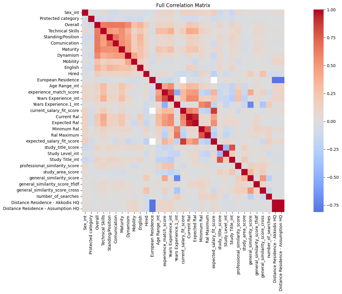
df_corr = dataset[columns_to_keep].copy()

bool_cols = df_corr.select_dtypes(include='bool').columns
df_corr[bool_cols] = df_corr[bool_cols].astype(int)

df_corr_numeric = df_corr.select_dtypes(include=[np.number])

plt.figure(figsize=(20, 10))
sns.heatmap(df_corr_numeric.corr(), annot=False, 
              cmap="coolwarm", center=0, square=True)
plt.title("Full Correlation Matrix")
plt.tight_layout()
plt.show()

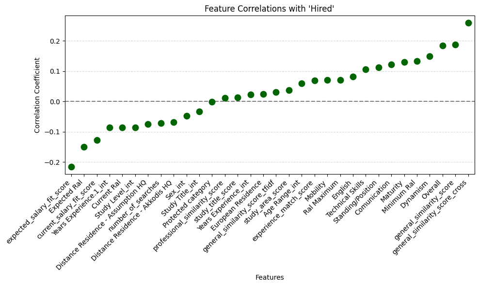
correlations = df_corr_numeric.corr()['Hired'].drop('Hired').sort_values()

plt.figure(figsize=(10, 6))
sns.stripplot(y=correlations.values, x=correlations.index, color='darkgreen', size=10)
plt.axhline(0, color='gray', linestyle='--')
plt.title("Feature Correlations with 'Hired'")
plt.ylabel("Correlation Coefficient")
plt.xlabel("Features")
plt.xticks(rotation=45, ha='right')
plt.grid(True, axis='y', linestyle='--', alpha=0.5)
plt.tight_layout()
plt.show()

print("Hiring Rate by Sex:")
distribution_by_sex = dataset.groupby('Sex')['Hired'].mean()
print(distribution_by_sex)

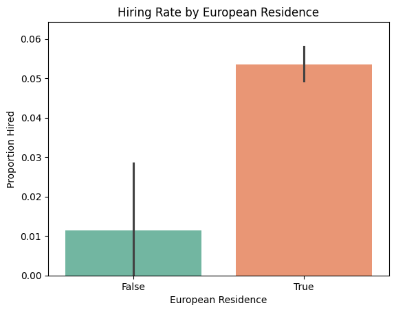
print("Hiring Rate by European Residence:")
distribution_by_eu_residence = dataset.groupby('European Residence')['Hired'].mean()
print(distribution_by_eu_residence)

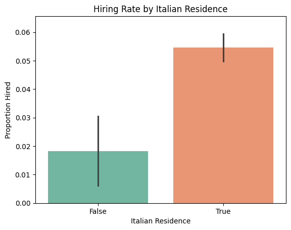
print("Hiring Rate by Italian Residence:")
distribution_by_it_residence = dataset.groupby('Italian Residence')['Hired'].mean()
print(distribution_by_it_residence)

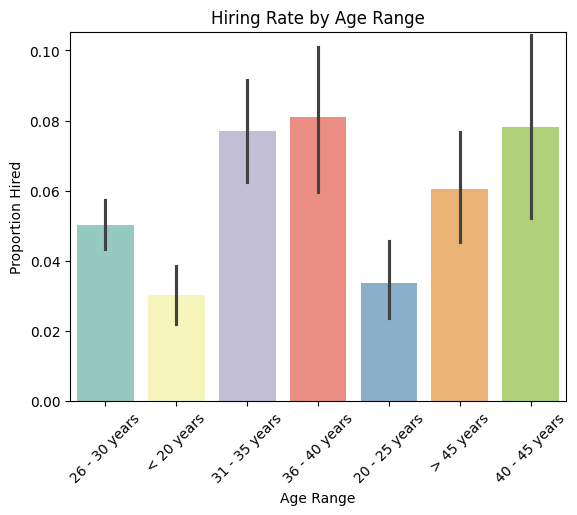
print("\nHiring Rate by Age Range:")
distribution_by_age = dataset.groupby('Age Range')['Hired'].mean()
print(distribution_by_age)

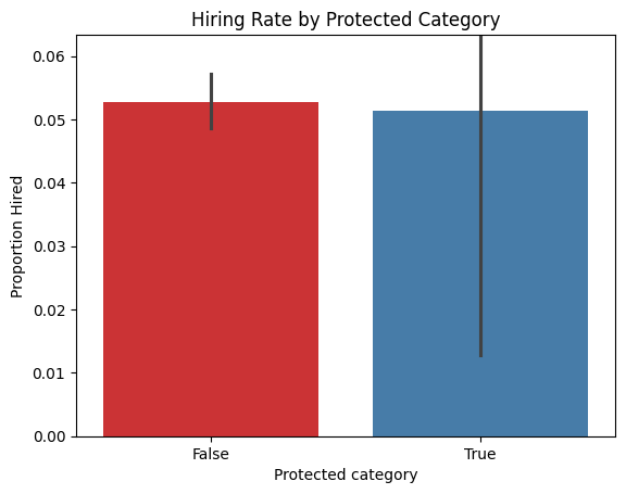
print("\nHiring Rate by Protected Category:")
distribution_by_category = dataset.groupby('Protected category')['Hired'].mean()
print(distribution_by_category)

sns.barplot(x='Sex', y='Hired', data=dataset, estimator=np.mean, palette='Set2')
plt.title("Hiring Rate by Sex")
plt.ylim(0, 1.2 * max(distribution_by_sex))
plt.ylabel("Proportion Hired")
plt.show()

sns.barplot(x='European Residence', y='Hired', data=dataset, estimator=np.mean, palette='Set2')
plt.title("Hiring Rate by European Residence")
plt.ylim(0, 1.2 * max(distribution_by_eu_residence))
plt.ylabel("Proportion Hired")
plt.show()

sns.barplot(x='Italian Residence', y='Hired', data=dataset, estimator=np.mean, palette='Set2')
plt.title("Hiring Rate by Italian Residence")
plt.ylim(0, 1.2 * max(distribution_by_it_residence))
plt.ylabel("Proportion Hired")
plt.show()

sns.barplot(x='Age Range', y='Hired', data=dataset, estimator=np.mean, palette='Set3')
plt.title("Hiring Rate by Age Range")
plt.ylim(0, 1.3 * max(distribution_by_age))
plt.xticks(rotation=45)
plt.ylabel("Proportion Hired")
plt.show()

sns.barplot(x='Protected category', y='Hired', data=dataset, estimator=np.mean, palette='Set1')
plt.title("Hiring Rate by Protected Category")
plt.ylim(0, 1.2 * max(distribution_by_category))
plt.ylabel("Proportion Hired")
plt.show()

Hiring Rate by Sex:
Sex
Female    0.073779
Male      0.047324
Name: Hired, dtype: float64
Hiring Rate by European Residence:
European Residence
False    0.011364
True     0.053534
Name: Hired, dtype: float64
Hiring Rate by Italian Residence:
Italian Residence
False    0.018293
True     0.054677
Name: Hired, dtype: float64

Hiring Rate by Age Range:
Age Range
20 - 25 years    0.033821
26 - 30 years    0.050131
31 - 35 years    0.077047
36 - 40 years    0.081040
40 - 45 years    0.078199
< 20 years       0.030227
> 45 years       0.060475
Name: Hired, dtype: float64

Hiring Rate by Protected Category:
Protected category
False    0.052784
True     0.051282
Name: Hired, dtype: float64

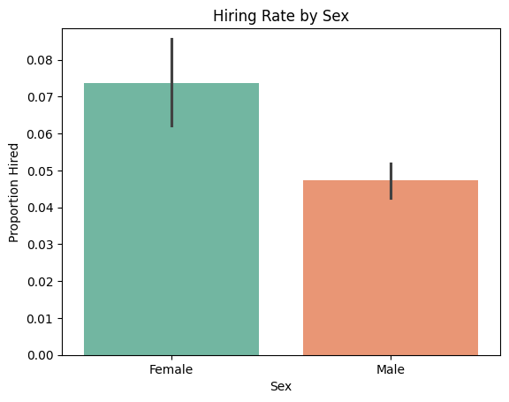
summary_sex = dataset.groupby('Sex')['Hired'].agg(['mean', 'count']).rename(columns={'mean': 'Hiring Rate', 'count': 'Number of Candidates'})
print("\nHiring Rate and Count by Sex:\n", summary_sex)

summary_eu_residence = dataset.groupby('European Residence')['Hired'].agg(['mean', 'count']).rename(columns={'mean': 'Hiring Rate', 'count': 'Number of Candidates'})
print("\nHiring Rate and Count by European Residence:\n", summary_eu_residence)

summary_it_residence = dataset.groupby('Italian Residence')['Hired'].agg(['mean', 'count']).rename(columns={'mean': 'Hiring Rate', 'count': 'Number of Candidates'})
print("\nHiring Rate and Count by Italian Residence:\n", summary_it_residence)

summary_age = dataset.groupby('Age Range')['Hired'].agg(['mean', 'count']).rename(columns={'mean': 'Hiring Rate', 'count': 'Number of Candidates'}).sort_index()
print("\nHiring Rate and Count by Age Range:\n", summary_age)

summary_protected = dataset.groupby('Protected category')['Hired'].agg(['mean', 'count']).rename(columns={'mean': 'Hiring Rate', 'count': 'Number of Candidates'})
print("\nHiring Rate and Count by Protected Category:\n", summary_protected)

Hiring Rate and Count by Sex:
         Hiring Rate  Number of Candidates
Sex                                      
Female     0.073779                  2006
Male       0.047324                  7734

Hiring Rate and Count by European Residence:
                     Hiring Rate  Number of Candidates
European Residence                                   
False                  0.011364                   176
True                   0.053534                  9564

Hiring Rate and Count by Italian Residence:
                    Hiring Rate  Number of Candidates
Italian Residence                                   
False                 0.018293                   492
True                  0.054677                  9236

Hiring Rate and Count by Age Range:
                Hiring Rate  Number of Candidates
Age Range                                       
20 - 25 years     0.033821                  1094
26 - 30 years     0.050131                  3810
31 - 35 years     0.077047                  1246
36 - 40 years     0.081040                   654
40 - 45 years     0.078199                   422
< 20 years        0.030227                  1588
> 45 years        0.060475                   926

Hiring Rate and Count by Protected Category:
                     Hiring Rate  Number of Candidates
Protected category                                   
False                  0.052784                  9662
True                   0.051282                    78

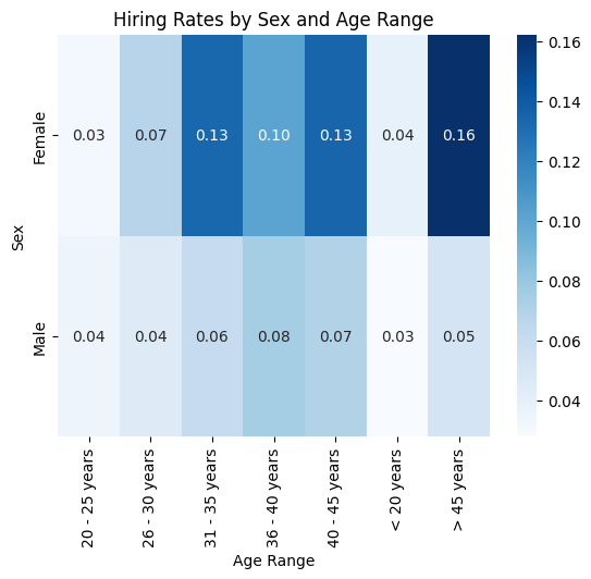
intersection = dataset.groupby(['Sex', 'Age Range'])['Hired'].mean().unstack()
print("\nHiring Rate by Sex and Age Range:")
print(intersection)

sns.heatmap(intersection, annot=True, cmap='Blues', fmt=".2f")
plt.title("Hiring Rates by Sex and Age Range")
plt.ylabel("Sex")
plt.xlabel("Age Range")
plt.show()

Hiring Rate by Sex and Age Range:
Age Range  20 - 25 years  26 - 30 years  31 - 35 years  36 - 40 years  \
Sex                                                                     
Female          0.030612       0.068235       0.133588       0.101449   
Male            0.035000       0.044932       0.061992       0.075581   

Age Range  40 - 45 years  < 20 years  > 45 years  
Sex                                               
Female          0.134615    0.038690    0.162162  
Male            0.070270    0.027955    0.051643  

p_selected_female = dataset[dataset['Sex'] == 'Female']['Hired'].mean()
p_selected_male = dataset[dataset['Sex'] == 'Male']['Hired'].mean()

disparate_impact = p_selected_female / p_selected_male
print("\nDisparate Impact Ratio (Female vs Male):", round(disparate_impact, 3))

Disparate Impact Ratio (Female vs Male): 1.559

Analysis of Hiring Rates

1. Gender (Sex) Females are hired at a significantly higher rate than males, suggesting a possible organizational emphasis on gender diversity or a potential bias favoring female candidates.

2. Age Range Hiring rates increase with age, peaking between 31–45 years, indicating a clear preference for mid-career professionals with more experience. Younger candidates, especially under 26, face notably lower hiring chances.

3. European Residence Candidates residing in Europe are far more likely to be hired, which may reflect logistical preferences, legal work eligibility, or alignment with company locations and operations.

4. Italian Residence There is a strong hiring bias toward candidates living in Italy. This suggests the organization prefers local hires, potentially to reduce relocation costs or due to legal/employment constraints.

5. Protected Category No meaningful difference in hiring rates between protected and non-protected groups was found. However, due to the very small sample of protected category candidates, no reliable conclusion can be drawn.

Drop Nan Values

import pandas as pd

df = dataset.copy()

print(f"{'Column':30} | {'Rows Before':10} | {'Rows After':10} | {'Hired Before':12} | {'Hired After':11} | {'% Hired Before':14} | {'% Hired After':13}")
print("-" * 105)

rows_before = len(df)
hired_before = df['Hired'].sum()
perc_hired_before = hired_before / rows_before * 100

for col in columns_to_keep:
    df_dropped = df.dropna(subset=[col])
    
    rows_after = len(df_dropped)
    hired_after = df_dropped['Hired'].sum()
    
    perc_hired_after = hired_after / rows_after * 100 if rows_after > 0 else 0
    
    print(f"{col:30} | {rows_before:<10} | {rows_after:<10} | {hired_before:<12} | {hired_after:<11} | {perc_hired_before:<14.2f} | {perc_hired_after:<13.2f}")

Column                         | Rows Before | Rows After | Hired Before | Hired After | % Hired Before | % Hired After
---------------------------------------------------------------------------------------------------------
Sex_int                        | 9740       | 9740       | 514          | 514         | 5.28           | 5.28         
Protected category             | 9740       | 9740       | 514          | 514         | 5.28           | 5.28         
Overall                        | 9740       | 4410       | 514          | 509         | 5.28           | 11.54        
Technical Skills               | 9740       | 4398       | 514          | 509         | 5.28           | 11.57        
Standing/Position              | 9740       | 4398       | 514          | 509         | 5.28           | 11.57        
Comunication                   | 9740       | 4398       | 514          | 509         | 5.28           | 11.57        
Maturity                       | 9740       | 4398       | 514          | 509         | 5.28           | 11.57        
Dynamism                       | 9740       | 4396       | 514          | 509         | 5.28           | 11.58        
Mobility                       | 9740       | 4396       | 514          | 509         | 5.28           | 11.58        
English                        | 9740       | 4390       | 514          | 509         | 5.28           | 11.59        
Hired                          | 9740       | 9740       | 514          | 514         | 5.28           | 5.28         
Italian Residence              | 9740       | 9728       | 514          | 514         | 5.28           | 5.28         
European Residence             | 9740       | 9740       | 514          | 514         | 5.28           | 5.28         
Age Range_int                  | 9740       | 9740       | 514          | 514         | 5.28           | 5.28         
experience_match_score         | 9740       | 9740       | 514          | 514         | 5.28           | 5.28         
Years Experience_int           | 9740       | 9740       | 514          | 514         | 5.28           | 5.28         
Years Experience.1_int         | 9740       | 9740       | 514          | 514         | 5.28           | 5.28         
current_salary_fit_score       | 9740       | 269        | 514          | 68          | 5.28           | 25.28        
Current Ral                    | 9740       | 1280       | 514          | 133         | 5.28           | 10.39        
Expected Ral                   | 9740       | 1144       | 514          | 149         | 5.28           | 13.02        
Minimum Ral                    | 9740       | 1733       | 514          | 237         | 5.28           | 13.68        
Ral Maximum                    | 9740       | 2526       | 514          | 310         | 5.28           | 12.27        
expected_salary_fit_score      | 9740       | 240        | 514          | 82          | 5.28           | 34.17        
study_title_score              | 9740       | 4725       | 514          | 438         | 5.28           | 9.27         
Study Level_int                | 9740       | 4725       | 514          | 438         | 5.28           | 9.27         
Study Title_int                | 9740       | 9740       | 514          | 514         | 5.28           | 5.28         
professional_similarity_score  | 9740       | 4425       | 514          | 471         | 5.28           | 10.64        
study_area_score               | 9740       | 4725       | 514          | 438         | 5.28           | 9.27         
general_similarity_score       | 9740       | 9740       | 514          | 514         | 5.28           | 5.28         
general_similarity_score_tfidf | 9740       | 9740       | 514          | 514         | 5.28           | 5.28         
general_similarity_score_cross | 9740       | 9740       | 514          | 514         | 5.28           | 5.28         
number_of_searches             | 9740       | 9735       | 514          | 509         | 5.28           | 5.23         
Distance Residence - Akkodis HQ | 9740       | 4724       | 514          | 438         | 5.28           | 9.27         
Distance Residence - Assumption HQ | 9740       | 4894       | 514          | 510         | 5.28           | 10.42        

df_cleaned = dataset.dropna(subset=[ 'professional_similarity_score', ])

print(f"Original data shape: {dataset.shape,(dataset['Hired']==True).sum()}")
print(f"Cleaned data shape: {df_cleaned.shape,(df_cleaned['Hired']==True).sum()}")

Original data shape: ((9740, 58), np.int64(514))
Cleaned data shape: ((4425, 58), np.int64(471))

Save Cleaned Dataset

df_cleaned.to_csv('cleaned_dataset.csv', index=False)

Training

Load Cleaned Dataset

import pandas as pd

df_cleaned = pd.read_csv('cleaned_dataset.csv')

Models Comparison

import pandas as pd
import numpy as np
import matplotlib.pyplot as plt
import seaborn as sns

from sklearn.model_selection import train_test_split
from sklearn.metrics import f1_score, accuracy_score, precision_score, recall_score
from sklearn.ensemble import RandomForestClassifier, HistGradientBoostingClassifier, VotingClassifier
from sklearn.linear_model import LogisticRegression
from sklearn.neural_network import MLPClassifier
from sklearn.preprocessing import StandardScaler
from sklearn.impute import SimpleImputer

from xgboost import XGBClassifier
from lightgbm import LGBMClassifier
from catboost import CatBoostClassifier

from imblearn.over_sampling import SMOTE, ADASYN
from imblearn.under_sampling import RandomUnderSampler
from imblearn.ensemble import BalancedRandomForestClassifier

random_state = 42

df = df_cleaned[columns_to_keep].copy()
X = df.drop(columns=['Hired'])
y = df['Hired']

bool_cols = X.select_dtypes(include='bool').columns
non_bool_cols = [c for c in X.columns.difference(bool_cols) if c != 'Sex_int']
X[bool_cols] = X[bool_cols].astype(int)

X_train, X_test, y_train, y_test = train_test_split(X, y, stratify=y, test_size=0.2, random_state=random_state)
scaler = StandardScaler()
X_train[non_bool_cols] = scaler.fit_transform(X_train[non_bool_cols])
X_test[non_bool_cols] = scaler.transform(X_test[non_bool_cols])
imputer = SimpleImputer(strategy='mean')
X_train_imputed = pd.DataFrame(imputer.fit_transform(X_train), columns=X_train.columns)
X_test_imputed = pd.DataFrame(imputer.transform(X_test), columns=X_test.columns)

X_train_upsampled, y_train_upsampled = ADASYN(random_state=random_state).fit_resample(X_train_imputed, y_train)
downsampler_impl = RandomUnderSampler(sampling_strategy='majority', random_state=random_state)
X_train_downsampled, y_train_downsampled = downsampler_impl.fit_resample(X_train_imputed, y_train)

models = {
    'RandomForest': lambda: RandomForestClassifier(class_weight='balanced', random_state=random_state, max_depth=10, min_samples_split=5, n_estimators=100),
    'HistGradientBoosting': lambda: HistGradientBoostingClassifier(random_state=random_state),
    'XGBoost': lambda: XGBClassifier(scale_pos_weight=(y_train == 0).sum() / (y_train == 1).sum(), random_state=random_state, eval_metric='logloss', max_depth=6),
    'LightGBM': lambda: LGBMClassifier(class_weight='balanced', random_state=random_state, max_depth=6, min_data_in_leaf=20, verbosity=-1),
    'LogisticRegression': lambda: LogisticRegression(class_weight='balanced', max_iter=1000, penalty='l2', C=0.1, solver='liblinear', random_state=random_state),
    'CatBoost': lambda: CatBoostClassifier(auto_class_weights='Balanced', silent=True, random_state=random_state, l2_leaf_reg=3, iterations=500, depth=6, learning_rate=0.05),
    'BalancedRF': lambda: BalancedRandomForestClassifier(random_state=random_state)
}

ensemble = lambda: VotingClassifier(
    estimators=[
        ('xgb', models['XGBoost']()),
        ('lgbm', models['LightGBM']()),
        ('cat', models['CatBoost']()),
        ('hist', models['HistGradientBoosting']()),
        ('brf', models['BalancedRF']())
    ],
    voting='soft'
)
models['Ensemble'] = ensemble

results_train = {}
results_test = {}

for strategy_name in ['Downsample', 'Original', 'Upsample']:
    strategy_results_train = []
    strategy_results_test = []
    
    for model_name, model in models.items():
        model = model()
        if strategy_name == 'Original':
            if model_name in ['XGBoost', 'LightGBM', 'CatBoost']:
                X_tr = X_train
                y_tr = y_train
                X_te = X_test
            else:
                X_tr = X_train_imputed
                y_tr = y_train
                X_te = X_test_imputed
        elif strategy_name == 'Upsample':
            X_tr = X_train_upsampled
            y_tr = y_train_upsampled
            X_te = X_test_imputed
        elif strategy_name == 'Downsample':
            X_tr = X_train_downsampled
            y_tr = y_train_downsampled
            X_te = X_test_imputed  
    
        model.fit(X_tr, y_tr)
        y_pred_train = model.predict(X_tr)
        y_pred_test = model.predict(X_te)
        
        strategy_results_train.append([
            model_name,
            f1_score(y_tr, y_pred_train),
            accuracy_score(y_tr, y_pred_train),
            precision_score(y_tr, y_pred_train),
            recall_score(y_tr, y_pred_train)
        ])
        
        strategy_results_test.append([
            model_name,
            f1_score(y_test, y_pred_test),
            accuracy_score(y_test, y_pred_test),
            precision_score(y_test, y_pred_test),
            recall_score(y_test, y_pred_test)
        ])
    
    results_train[strategy_name] = pd.DataFrame(strategy_results_train, columns=['Model', 'F1 Score', 'Accuracy', 'Precision', 'Recall'])
    results_test[strategy_name] = pd.DataFrame(strategy_results_test, columns=['Model', 'F1 Score', 'Accuracy', 'Precision', 'Recall'])

print("\nTraining Data Results:")
for strategy_name, result_df in results_train.items():
    print(f"\nResults for {strategy_name} Sampling (Training Data):")
    print(result_df.sort_values(by='F1 Score', ascending=False).to_string(index=False))

print("\nTest Data Results:")
for strategy_name, result_df in results_test.items():
    print(f"\nResults for {strategy_name} Sampling (Test Data):")
    print(result_df.sort_values(by='F1 Score', ascending=False).to_string(index=False))

strategy_colors = {
    'Original': sns.color_palette("tab10")[0],
    'Upsample': sns.color_palette("tab10")[1],
    'Downsample': sns.color_palette("tab10")[2],
}

plt.figure(figsize=(12, 8))

for strategy_name, result_df in results_test.items():
    color = strategy_colors[strategy_name]
    plt.plot(result_df['Model'], result_df['F1 Score'], label=f"{strategy_name} (Test)", marker='o', linestyle='--', color=color)

for strategy_name, result_df in results_train.items():
    color = strategy_colors[strategy_name]
    plt.plot(result_df['Model'], result_df['F1 Score'], label=f"{strategy_name} (Train)", marker='o', linestyle='-', color=color)

plt.title('F1 Score Comparison Across Strategies (Train vs Test)')
plt.ylabel('F1 Score')
plt.xlabel('Models')
plt.xticks(rotation=45)
plt.legend()
plt.grid(True)
plt.tight_layout()
plt.show()

Training Data Results:

Results for Downsample Sampling (Training Data):
               Model  F1 Score  Accuracy  Precision   Recall
HistGradientBoosting  1.000000  1.000000   1.000000 1.000000
             XGBoost  1.000000  1.000000   1.000000 1.000000
            LightGBM  1.000000  1.000000   1.000000 1.000000
            CatBoost  1.000000  1.000000   1.000000 1.000000
            Ensemble  1.000000  1.000000   1.000000 1.000000
          BalancedRF  1.000000  1.000000   1.000000 1.000000
        RandomForest  0.990777  0.990716   0.984293 0.997347
  LogisticRegression  0.780952  0.786472   0.801676 0.761273

Results for Original Sampling (Training Data):
               Model  F1 Score  Accuracy  Precision   Recall
HistGradientBoosting  1.000000  1.000000   1.000000 1.000000
             XGBoost  1.000000  1.000000   1.000000 1.000000
            Ensemble  0.998675  0.999718   0.997354 1.000000
            CatBoost  0.993412  0.998589   0.986911 1.000000
            LightGBM  0.979221  0.995485   0.959288 1.000000
        RandomForest  0.921569  0.981941   0.856492 0.997347
          BalancedRF  0.748759  0.928612   0.598413 1.000000
  LogisticRegression  0.462758  0.808691   0.329944 0.774536

Results for Upsample Sampling (Training Data):
               Model  F1 Score  Accuracy  Precision   Recall
HistGradientBoosting  1.000000  1.000000   1.000000 1.000000
             XGBoost  1.000000  1.000000   1.000000 1.000000
          BalancedRF  1.000000  1.000000   1.000000 1.000000
            Ensemble  1.000000  1.000000   1.000000 1.000000
            CatBoost  0.999841  0.999841   1.000000 0.999681
            LightGBM  0.999841  0.999841   1.000000 0.999681
        RandomForest  0.987222  0.987155   0.977812 0.996814
  LogisticRegression  0.775504  0.779099   0.784736 0.766486

Test Data Results:

Results for Downsample Sampling (Test Data):
               Model  F1 Score  Accuracy  Precision   Recall
            LightGBM  0.640000  0.888388   0.486188 0.936170
            CatBoost  0.634146  0.881623   0.471503 0.968085
HistGradientBoosting  0.623656  0.881623   0.470270 0.925532
            Ensemble  0.619718  0.878241   0.463158 0.936170
          BalancedRF  0.605263  0.864713   0.438095 0.978723
        RandomForest  0.588608  0.853439   0.418919 0.989362
             XGBoost  0.582781  0.857948   0.423077 0.936170
  LogisticRegression  0.446541  0.801578   0.316964 0.755319

Results for Original Sampling (Test Data):
               Model  F1 Score  Accuracy  Precision   Recall
            Ensemble  0.795812  0.956032   0.783505 0.808511
            CatBoost  0.793970  0.953777   0.752381 0.840426
HistGradientBoosting  0.776471  0.957159   0.868421 0.702128
             XGBoost  0.774194  0.952649   0.782609 0.765957
            LightGBM  0.763285  0.944758   0.699115 0.840426
        RandomForest  0.731959  0.941375   0.710000 0.755319
          BalancedRF  0.676806  0.904171   0.526627 0.946809
  LogisticRegression  0.472131  0.818489   0.341232 0.765957

Results for Upsample Sampling (Test Data):
               Model  F1 Score  Accuracy  Precision   Recall
            LightGBM  0.778947  0.952649   0.770833 0.787234
            Ensemble  0.778947  0.952649   0.770833 0.787234
HistGradientBoosting  0.761905  0.949267   0.757895 0.765957
            CatBoost  0.756757  0.949267   0.769231 0.744681
             XGBoost  0.742268  0.943630   0.720000 0.765957
          BalancedRF  0.733668  0.940248   0.695238 0.776596
        RandomForest  0.731481  0.934611   0.647541 0.840426
  LogisticRegression  0.452012  0.800451   0.318777 0.776596

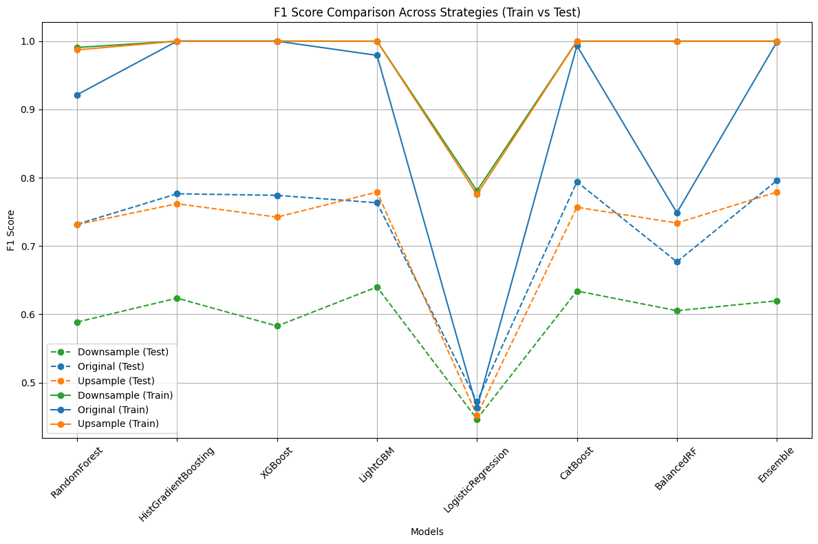
Summary

• Ensemble consistently outperforms other models on test data across all sampling strategies, achieving the highest F1 scores (up to 0.80 with original dataset).

• LightGBM, HistGradientBoosting, XGBoost and CatBoost models also perform well, particularly with original and upsampled data.

• RandomForest and BalancedRF show solid performance but slightly trail behind the top models.

• BalancedRF benefits most from upsampling but underperforms with original and downsampled data.

• Logistic Regression lags across all settings, confirming that more complex models handle the task better.

All models show perfect or near-perfect results on training data, indicating clear overfitting, likely due to the limited dataset size.

Features Removal Comparison

from tqdm import tqdm
from sklearn.metrics import f1_score

def compare_feature_sets(feature_sets, test_models):
    results = []

    for feat_set_name, feat_cols in tqdm(feature_sets.items(), desc='Feature sets'):
        X_sub = df_cleaned[feat_cols].copy()
        y_sub = df_cleaned['Hired']

        bool_cols = X_sub.select_dtypes(include='bool').columns
        non_bool_cols = X_sub.columns.difference(bool_cols)

        X_sub[bool_cols] = X_sub[bool_cols].astype(int)

        X_train, X_test, y_train, y_test = train_test_split(
            X_sub, y_sub, stratify=y_sub, test_size=0.2, random_state=random_state
        ) 
        scaler = StandardScaler()
        X_train[non_bool_cols] = scaler.fit_transform(X_train[non_bool_cols])
        X_test[non_bool_cols] = scaler.transform(X_test[non_bool_cols])
        imputer = SimpleImputer(strategy='mean')
        X_train_imputed = pd.DataFrame(imputer.fit_transform(X_train), columns=X_train.columns)
        X_test_imputed = pd.DataFrame(imputer.transform(X_test), columns=X_test.columns)

        for model_name, model_lambda in test_models.items():
            model = model_lambda()
            if model_name in ['LightGBM', 'CatBoost']:
                X_tr = X_train
                X_te = X_test
            else:
                X_tr = X_train_imputed
                X_te = X_test_imputed
            model.fit(X_tr, y_train)
            y_pred_test = model.predict(X_te)
            y_pred_train = model.predict(X_tr)
            f1_test = f1_score(y_test, y_pred_test)
            f1_train = f1_score(y_train, y_pred_train)
            results.append({
                'Feature Set': feat_set_name,
                'Model': model_name,
                'Train F1': f1_train,
                'Test F1': f1_test
            })

    results_df = pd.DataFrame(results)

    best_row = results_df.loc[results_df['Test F1'].idxmax()]
    print(f"\nBest performance:\nFeature Set: {best_row['Feature Set']}, Model: {best_row['Model']}, F1 Score: {best_row['Test F1']:.4f}")
    return results_df

feature_columns = [col for col in columns_to_keep if col != 'Hired']

feature_sets = {
    'general_similarity_score_cross': [col for col in feature_columns if col not in ['general_similarity_score', 'general_similarity_score_tfidf']],
    'general_similarity_score': [col for col in feature_columns if col not in ['general_similarity_score_tfidf', 'general_similarity_score_cross']],
    'general_similarity_score_tfidf': [col for col in feature_columns if col not in ['general_similarity_score', 'general_similarity_score_cross']],
    'None ':  [col for col in feature_columns if col not in ['general_similarity_score_tfidf', 'general_similarity_score', 'general_similarity_score_cross']], 
    'all': feature_columns,
    }

test_models = {
    "LightGBM":models['LightGBM'],
    'CatBoost': models['CatBoost'],
    'Ensemble': models['Ensemble'],
}

results_df = compare_feature_sets(feature_sets, test_models)
results_df

Feature sets: 100%|██████████| 5/5 [00:24<00:00,  4.85s/it]

Best performance:
Feature Set: general_similarity_score, Model: Ensemble, F1 Score: 0.7959

	Feature Set	Model	Train F1	Test F1
0	general_similarity_score_cross	LightGBM	0.946048	0.767773
1	general_similarity_score_cross	CatBoost	0.977951	0.766990
2	general_similarity_score_cross	Ensemble	0.994723	0.766169
3	general_similarity_score	LightGBM	0.959288	0.759259
4	general_similarity_score	CatBoost	0.994723	0.766169
5	general_similarity_score	Ensemble	0.997354	0.795918
6	general_similarity_score_tfidf	LightGBM	0.919512	0.745455
7	general_similarity_score_tfidf	CatBoost	0.976684	0.751220
8	general_similarity_score_tfidf	Ensemble	0.996037	0.790244
9	None	LightGBM	0.930864	0.745455
10	None	CatBoost	0.975420	0.768519
11	None	Ensemble	0.994723	0.775120
12	all	LightGBM	0.979221	0.763285
13	all	CatBoost	0.993412	0.793970
14	all	Ensemble	0.998675	0.795812

plt.figure(figsize=(12, 6))
sns.barplot(data=results_df, x="Feature Set", y="Test F1", hue="Model")
plt.xticks(rotation=45, ha="right")
plt.ylim(0.8*min(results_df['Test F1']))
plt.title("F1 Scores by Feature Set and Model")
plt.tight_layout()
plt.legend(title="Model")
plt.grid(axis='y')

plt.show()

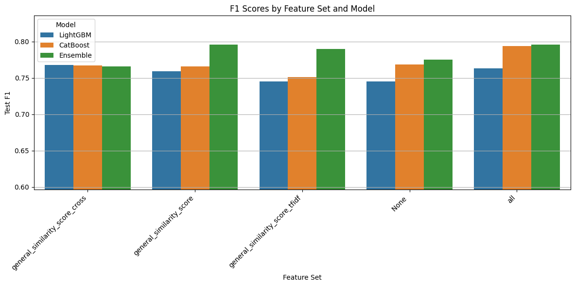
Feature Set Comparison Summary

The best performance (F1 = 0.796) was achieved using only the general_similarity_score feature with the Ensemble model. This suggests that deep semantic similarity captured through a bi-encoder model can provide a highly effective signal for predicting hires, even if it’s not consistently the best across all models.

• general_similarity_score uses a SentenceTransformer encoder and cosine similarity to capture deep semantic relationships.

• general_similarity_score_cross leverages a cross-encoder transformer that jointly processes candidate and job texts, allowing for nuanced contextual matching.

• general_similarity_score_tfidf calculates cosine similarity between TF-IDF vectors, highlighting surface-level lexical overlap.

Both the general_similarity_score_cross and all feature sets also produced strong and consistent results across multiple models, demonstrating the robustness of combining similarity signals. In particular, general_similarity_score_cross often yielded reliable performance, though it did not outperform the peak result from general_similarity_score with the Ensemble model.

Notably, excluding all similarity features leads to a significant drop in F1 (e.g., Ensemble F1 falls to 0.775), emphasizing the importance of text similarity for this task.

Given that general_similarity_score achieves the highest single F1 score, even if not consistently the best across all settings, we opt to use only general_similarity_score in the final model. This choice balances performance with simplicity and computational efficiency, while capturing the strongest individual signal observed.

feature_sets = {
    "base_attributes": [
        "Sex_int",
        "Protected category",
        "Overall",
        "Technical Skills",
        "Standing/Position",
        "Comunication",
        "Maturity",
        "Dynamism",
        "Mobility",
        "English",
        "Italian Residence",
        "European Residence",
        "Age Range_int",
        "Years Experience_int",
        "Years Experience.1_int",
        "Current Ral",
        "Expected Ral",
        "Minimum Ral",
        "Ral Maximum",
        "Study Level_int",
        "Study Title_int",
        "number_of_searches",
    ],
    "custom_scores": [
        "experience_match_score",
        "current_salary_fit_score",
        "expected_salary_fit_score",
        "study_title_score",
        "professional_similarity_score",
        "study_area_score",
        "general_similarity_score",
        "Distance Residence - Akkodis HQ",
        "Distance Residence - Assumption HQ",
    ],
    "custom_scores_with_essential_base_attributes": [
        # Base Attributes
        "Sex_int",
        "Protected category",
        "Overall",
        "Technical Skills",
        "Standing/Position",
        "Comunication",
        "Maturity",
        "Dynamism",
        "Mobility",
        "English",
        "Italian Residence",
        "European Residence",
        "Age Range_int",
        "number_of_searches",
        # Custom Similarity Scores
        "experience_match_score",
        "current_salary_fit_score",
        "expected_salary_fit_score",
        "study_title_score",
        "professional_similarity_score",
        "study_area_score",
        "general_similarity_score",
        "Distance Residence - Akkodis HQ",
        "Distance Residence - Assumption HQ",
    ],
    "base_attributes_with_essential_custom_scores": [
        # Base Attributes
        "Sex_int",
        "Protected category",
        "Overall",
        "Technical Skills",
        "Standing/Position",
        "Comunication",
        "Maturity",
        "Dynamism",
        "Mobility",
        "English",
        "Italian Residence",
        "European Residence",
        "Age Range_int",
        "number_of_searches",
        # Essential Custom Similarity Scores
        "study_area_score",
        "general_similarity_score",
        "Distance Residence - Akkodis HQ",
        "Distance Residence - Assumption HQ",
        # Additional Base Attributes
        "Years Experience_int",
        "Years Experience.1_int",
        "Current Ral",
        "Expected Ral",
        "Minimum Ral",
        "Ral Maximum",
        "Study Level_int",
        "Study Title_int",
    ],
    "all": [
        # Base Attributes
        "Sex_int",
        "Protected category",
        "Overall",
        "Technical Skills",
        "Standing/Position",
        "Comunication",
        "Maturity",
        "Dynamism",
        "Mobility",
        "English",
        "Italian Residence",
        "European Residence",
        "Age Range_int",
        "number_of_searches", 
        # Custom Similarity Scores
        "experience_match_score",
        "expected_salary_fit_score",
        "current_salary_fit_score",
        "professional_similarity_score",
        "study_area_score",
        "general_similarity_score",
        "study_title_score",
        "Distance Residence - Akkodis HQ",
        "Distance Residence - Assumption HQ",
        # Additional Base Attributes
        "Years Experience_int",
        "Years Experience.1_int",
        "Current Ral",
        "Expected Ral",
        "Minimum Ral",
        "Ral Maximum",
        "Study Level_int",
        "Study Title_int",  
    ],
}
results_df = compare_feature_sets(feature_sets, test_models)
results_df

Feature sets: 100%|██████████| 5/5 [00:23<00:00,  4.79s/it]

Best performance:
Feature Set: all, Model: CatBoost, F1 Score: 0.8079

	Feature Set	Model	Train F1	Test F1
0	base_attributes	LightGBM	0.826754	0.700422
1	base_attributes	CatBoost	0.943680	0.700935
2	base_attributes	Ensemble	0.970399	0.695238
3	custom_scores	LightGBM	0.798694	0.525424
4	custom_scores	CatBoost	0.892308	0.480769
5	custom_scores	Ensemble	0.954430	0.510638
6	custom_scores_with_essential_base_attributes	LightGBM	0.933168	0.767123
7	custom_scores_with_essential_base_attributes	CatBoost	0.990802	0.790244
8	custom_scores_with_essential_base_attributes	Ensemble	0.996037	0.800000
9	base_attributes_with_essential_custom_scores	LightGBM	0.955640	0.739336
10	base_attributes_with_essential_custom_scores	CatBoost	0.990802	0.788177
11	base_attributes_with_essential_custom_scores	Ensemble	0.997354	0.797927
12	all	LightGBM	0.966667	0.768519
13	all	CatBoost	0.988204	0.807882
14	all	Ensemble	0.997354	0.802030

plt.figure(figsize=(12, 6))
sns.barplot(data=results_df, x="Feature Set", y="Test F1", hue="Model")
plt.xticks(rotation=45, ha="right")
plt.ylim(0.8*min(results_df['Test F1']))
plt.title("F1 Scores by Feature Set and Model")
plt.tight_layout()
plt.legend(title="Model")
plt.grid(axis='y')

plt.show()

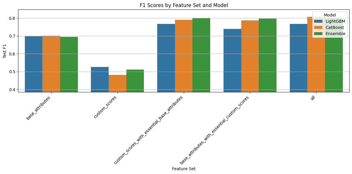
Feature Set Comparison Summary

The best performance is achieved with the all feature set using the CatBoost model, reaching a Test F1 Score of 0.8079.

Summary of the tested feature sets:

• base_attributes
  Encompasses a comprehensive set of features describing both the candidate (e.g., age, residence, language, education, experience) and the job requirements or evaluations (e.g., technical skills, position, salary ranges, overall fit scores).
  This foundational information captures the context of both parties but lacks direct indicators of compatibility between them. Performance is moderate as a result.

• custom_scores
  Focuses exclusively on engineered features that quantify the match between candidate and job — including salary fit, study alignment, professional similarity, and location distance.
  These scores alone underperform, suggesting that without descriptive context, match scores don’t provide enough standalone signal.

• custom_scores_with_essential_base_attributes
  Builds on the custom similarity scores by integrating critical base attributes that anchor the match in relevant candidate-job context (like key demographics and job-related features).
  This hybrid set performs very well, offering a balance between match precision and contextual understanding.

• base_attributes_with_essential_custom_scores
  Starts with a rich base attribute set and adds only the most important custom scores (e.g., general similarity, location distance).
  It effectively reinforces candidate-job context with minimal additional complexity, also producing strong results.

• all
  Combines every available feature into one comprehensive set — including all base attributes and all custom scores.
  While this approach slightly edges out others in performance, the marginal gain may not justify the added feature redundancy and risk of overfitting.

Conclusion: While the all feature set shows the highest F1 score, we select the custom_scores_with_essential_base_attributes feature set as the optimal choice. It provides nearly equivalent performance with fewer features, reducing complexity and redundancy. These results also highlight that:

• Base attributes alone are not sufficient, as they lack direct match indicators.

• Custom similarity scores alone are also insufficient, as they lack foundational context.

• The best results come from combining custom match scores with key descriptive features, ensuring both contextual grounding and match relevance.

Sampling Techniques

import pandas as pd
import numpy as np
import matplotlib.pyplot as plt
import seaborn as sns
from tqdm import tqdm
from sklearn.model_selection import train_test_split
from sklearn.metrics import f1_score
from sklearn.preprocessing import StandardScaler
from sklearn.impute import SimpleImputer

from catboost import CatBoostClassifier
from xgboost import XGBClassifier
from lightgbm import LGBMClassifier
from sklearn.ensemble import VotingClassifier

from imblearn.over_sampling import SMOTE, ADASYN, BorderlineSMOTE, SVMSMOTE
from imblearn.under_sampling import RandomUnderSampler


df = df_cleaned[feature_sets['custom_scores_with_essential_base_attributes']+['Hired']].copy()
X = df.drop(columns=['Hired'])
y = df['Hired']

bool_cols = X.select_dtypes(include='bool').columns
non_bool_cols = X.columns.difference(bool_cols)

X[bool_cols] = X[bool_cols].astype(int)


X_train, X_test, y_train, y_test = train_test_split(
    X, y, stratify=y, test_size=0.2, random_state=random_state
)
scaler = StandardScaler()
X_train[non_bool_cols] = scaler.fit_transform(X_train[non_bool_cols])
X_test[non_bool_cols] = scaler.transform(X_test[non_bool_cols])

imputer = SimpleImputer(strategy='mean')
X_train_imputed = pd.DataFrame(imputer.fit_transform(X_train), columns=X_train.columns)
X_test_imputed = pd.DataFrame(imputer.transform(X_test), columns=X_test.columns)

X_orig, y_orig = X_train_imputed, y_train

minority_count = sum(y_orig == 1)
majority_count = sum(y_orig == 0)

smote_ratios = [0.25, 0.5, 0.75, 1.0]

resampled_datasets = {}

resampled_datasets['Original'] = {'imputed': (X_orig, y_orig, X_test_imputed), 'original': (X_train, y_train, X_test)}

for ratio in smote_ratios:
    name = f'SMOTE_{int(ratio*100)}%'
    smote = SMOTE(sampling_strategy=ratio, random_state=random_state)
    X_res, y_res = smote.fit_resample(X_orig, y_orig)
    resampled_datasets[name] = (X_res, y_res)

for ratio in smote_ratios:
    name = f'ADASYN_{int(ratio*100)}%'
    adasyn = ADASYN(sampling_strategy=ratio, random_state=random_state)
    X_res, y_res = adasyn.fit_resample(X_orig, y_orig)
    resampled_datasets[name] = (X_res, y_res)

for ratio in smote_ratios:
    name = f'BorderlineSMOTE_{int(ratio*100)}%'
    bl_smote = BorderlineSMOTE(sampling_strategy=ratio, random_state=random_state)
    X_res, y_res = bl_smote.fit_resample(X_orig, y_orig)
    resampled_datasets[name] = (X_res, y_res)

for ratio in smote_ratios:
    name = f'SVMSMOTE_{int(ratio*100)}%'
    svm_smote = SVMSMOTE(sampling_strategy=ratio, random_state=random_state)
    X_res, y_res = svm_smote.fit_resample(X_orig, y_orig)
    resampled_datasets[name] = (X_res, y_res)

resampled_datasets['Downsampling'] = RandomUnderSampler(random_state=random_state).fit_resample(X_orig, y_orig)

results = []

for strategy_name, trainset in tqdm(resampled_datasets.items(), desc='Training...'):
    for model_name, model_lambda in test_models.items():
        if strategy_name == 'Original':
            if model_name in ['LightGBM', 'CatBoost']:
                X_tr, y_tr, X_te = trainset['original']
            else: 
                X_tr, y_tr, X_te = trainset['imputed']
        else:
            (X_tr, y_tr) = trainset
            X_te = X_test_imputed
        model = model_lambda()
        model.fit(X_tr, y_tr)
        y_pred_test = model.predict(X_te)
        y_pred_train = model.predict(X_tr)
        f1_test = f1_score(y_test, y_pred_test)
        f1_train = f1_score(y_tr, y_pred_train)
        results.append({
            'Resampling': strategy_name,
            'Model': model_name,
            'Train F1': f1_train,
            'Test F1': f1_test
        })

results_df = pd.DataFrame(results)
results_df

Training...: 100%|██████████| 18/18 [02:26<00:00,  8.14s/it]

	Resampling	Model	Train F1	Test F1
0	Original	LightGBM	0.933168	0.767123
1	Original	CatBoost	0.990802	0.790244
2	Original	Ensemble	0.996037	0.800000
3	SMOTE_25%	LightGBM	0.977146	0.792453
4	SMOTE_25%	CatBoost	0.991850	0.780488
5	SMOTE_25%	Ensemble	0.999368	0.803922
6	SMOTE_50%	LightGBM	0.992774	0.800000
7	SMOTE_50%	CatBoost	0.998423	0.763819
8	SMOTE_50%	Ensemble	1.000000	0.800000
9	SMOTE_75%	LightGBM	0.995798	0.795918
10	SMOTE_75%	CatBoost	0.999369	0.791444
11	SMOTE_75%	Ensemble	1.000000	0.779487
12	SMOTE_100%	LightGBM	0.996687	0.781250
13	SMOTE_100%	CatBoost	0.999211	0.774194
14	SMOTE_100%	Ensemble	1.000000	0.783505
15	ADASYN_25%	LightGBM	0.970149	0.764151
16	ADASYN_25%	CatBoost	0.990305	0.780488
17	ADASYN_25%	Ensemble	0.997906	0.794118
18	ADASYN_50%	LightGBM	0.991558	0.790244
19	ADASYN_50%	CatBoost	0.997387	0.785714
20	ADASYN_50%	Ensemble	0.999673	0.796117
21	ADASYN_75%	LightGBM	0.996147	0.756477
22	ADASYN_75%	CatBoost	0.999142	0.771574
23	ADASYN_75%	Ensemble	1.000000	0.778325
24	ADASYN_100%	LightGBM	0.996505	0.779487
25	ADASYN_100%	CatBoost	0.998727	0.747368
26	ADASYN_100%	Ensemble	1.000000	0.781726
27	BorderlineSMOTE_25%	LightGBM	0.983219	0.813084
28	BorderlineSMOTE_25%	CatBoost	0.993719	0.796117
29	BorderlineSMOTE_25%	Ensemble	0.999368	0.811881
30	BorderlineSMOTE_50%	LightGBM	0.992453	0.803828
31	BorderlineSMOTE_50%	CatBoost	0.998422	0.806122
32	BorderlineSMOTE_50%	Ensemble	1.000000	0.807882
33	BorderlineSMOTE_75%	LightGBM	0.996845	0.810256
34	BorderlineSMOTE_75%	CatBoost	0.999579	0.802083
35	BorderlineSMOTE_75%	Ensemble	1.000000	0.804020
36	BorderlineSMOTE_100%	LightGBM	0.997789	0.776596
37	BorderlineSMOTE_100%	CatBoost	0.998736	0.753927
38	BorderlineSMOTE_100%	Ensemble	1.000000	0.797927
39	SVMSMOTE_25%	LightGBM	0.983219	0.786730
40	SVMSMOTE_25%	CatBoost	0.994343	0.794118
41	SVMSMOTE_25%	Ensemble	0.998737	0.817734
42	SVMSMOTE_50%	LightGBM	0.993390	0.793814
43	SVMSMOTE_50%	CatBoost	0.998107	0.791878
44	SVMSMOTE_50%	Ensemble	0.999684	0.816327
45	SVMSMOTE_75%	LightGBM	0.994747	0.822335
46	SVMSMOTE_75%	CatBoost	0.998527	0.800000
47	SVMSMOTE_75%	Ensemble	1.000000	0.824121
48	SVMSMOTE_100%	LightGBM	0.996845	0.816754
49	SVMSMOTE_100%	CatBoost	0.998895	0.774869
50	SVMSMOTE_100%	Ensemble	1.000000	0.824742
51	Downsampling	LightGBM	1.000000	0.644444
52	Downsampling	CatBoost	1.000000	0.644928
53	Downsampling	Ensemble	1.000000	0.626335

min_f1 = results_df['Test F1'].min()

plt.figure(figsize=(16, 8))
sns.barplot(
    data=results_df,
    x='Resampling',
    y='Test F1',
    hue='Model',
    palette='Set2'
)
plt.title('F1 Score of CatBoost, LightGBM and  Ensemble Models Across Resampling Techniques & Ratios')
plt.xticks(rotation=90)
plt.ylabel('F1 Score')
plt.ylim(bottom=0.95 * min_f1)
plt.xlabel('Resampling Strategy')
plt.legend(title='Model')
plt.tight_layout()
plt.show()

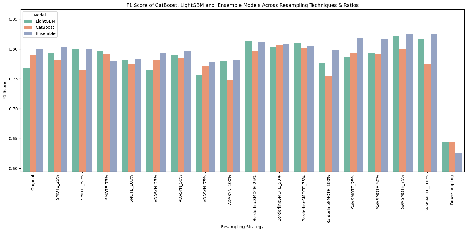
Resampling Strategy Comparison Summary

This experiment compared various resampling techniques to mitigate class imbalance, evaluating their impact on CatBoost, LightGBM, and Ensemble models based on Train and Test F1 scores.

Best Performance

• Top Result: SVMSMOTE_75% with Ensemble (Test F1 = 0.8241)

Final Choice: SMOTE_75%

We select SMOTE with 75% ratio as the preferred resampling strategy due to its strong performance and balanced data augmentation:

• Robust Test F1 Scores:

  • LightGBM F1 = 0.8223

  • CatBoost F1 = 0.8000

  • Ensemble F1 = 0.8241

• Improved Generalization compared to lower SMOTE ratios (25%, 50%) and original data.

• Controlled synthetic sample generation avoids overfitting seen at 100% oversampling levels.

How Sampling Ratio Affects Performance

• Original dataset (no resampling) provides a solid baseline with moderate test F1 scores (LightGBM: 0.7671, CatBoost: 0.7902, Ensemble: 0.8000), but the class imbalance limits further improvement.

• Lower SMOTE ratios (25%, 50%) improve Test F1 compared to the original dataset by alleviating class imbalance but may still under-represent the minority class, limiting gains.

• At 75% oversampling, the minority class is better represented, leading to improved model generalization and higher F1 scores across models.

• Increasing to 100% oversampling tends to introduce noise and redundancy in synthetic samples, causing slight performance drops, especially visible in CatBoost and Ensemble results.

• More complex resampling techniques like SVMSMOTE and BorderlineSMOTE show competitive or better performance at some ratios but come with increased computational cost and complexity.

Key Observations

• Original data shows that imbalance restricts maximum achievable performance despite strong training F1 scores.

• SMOTE_75% strikes the best balance between addressing class imbalance and avoiding overfitting or noise.

• SVMSMOTE_75% achieves the highest overall Test F1 with the Ensemble but at greater complexity.

• ADASYN methods deliver reasonable but less consistent results.

• Downsampling drastically reduces test performance despite perfect training scores, indicating overfitting.

Conclusion:
We select SMOTE with a 75% oversampling ratio as the optimal resampling strategy. It effectively balances minority class representation and avoids overfitting, leading to strong and consistent predictive performance across models while maintaining manageable computational costs.

Fairness Metrics

from catboost import CatBoostClassifier
from xgboost import XGBClassifier
from lightgbm import LGBMClassifier

from fairlearn.metrics import (
    MetricFrame,
    demographic_parity_difference,
    equalized_odds_difference
)
from sklearn.metrics import precision_score, recall_score
from sklearn.model_selection import train_test_split
from sklearn.impute import SimpleImputer
from sklearn.preprocessing import StandardScaler

import matplotlib.pyplot as plt
import seaborn as sns
import pandas as pd
import numpy as np

df = df_cleaned.copy()

protected_attributes = [
    'Sex_int', 'Protected category', 'Age Range_int',
    'Italian Residence', 'European Residence'
]

df = df.dropna(subset=protected_attributes).reset_index(drop=True)

X = df.drop(columns=['Hired'])[feature_sets['custom_scores_with_essential_base_attributes']]
y = df['Hired']

bool_cols = X.select_dtypes(include='bool').columns
non_bool_cols = X.columns.difference(bool_cols)

X[bool_cols] = X[bool_cols].astype(int)

X_train, X_test, y_train, y_test = train_test_split(X, y, stratify=y, test_size=0.2, random_state=random_state)

scaler = StandardScaler()
X_train[non_bool_cols] = scaler.fit_transform(X_train[non_bool_cols])
X_test[non_bool_cols] = scaler.transform(X_test[non_bool_cols])

imputer = SimpleImputer(strategy='mean')
X_train_imp = pd.DataFrame(imputer.fit_transform(X_train), columns=X.columns)
X_test_imp = pd.DataFrame(imputer.transform(X_test), columns=X.columns)

svm_smote = SMOTE(sampling_strategy=0.75, random_state=random_state)
X_res, y_res = svm_smote.fit_resample(X_train_imp, y_train)

majority_count = (y_res == 0).sum()
minority_count = (y_res == 1).sum()

catboost_model = models['CatBoost']()
lightgbm_model = models['LightGBM']()
ensemble_model = models['Ensemble']()

catboost_model.fit(X_res, y_res)
lightgbm_model.fit(X_res, y_res)
ensemble_model.fit(X_res, y_res)


y_pred_cat = catboost_model.predict(X_test_imp)
y_pred_lgb = lightgbm_model.predict(X_test_imp)
y_pred_ens = ensemble_model.predict(X_test_imp)

performance_results = []
fairness_results = []

for model_name, y_pred in [('CatBoost', y_pred_cat), ('LightGBM', y_pred_lgb), ('Ensemble', y_pred_ens)]:
    precision = precision_score(y_test, y_pred)
    recall = recall_score(y_test, y_pred)
    
    performance_results.append({
        'Model': model_name,
        'Precision': precision,
        'Recall': recall
    })
    
    for attr in protected_attributes:
        sensitive_features_test = dataset.loc[X_test.index, attr]
        dp_diff = demographic_parity_difference(
            y_true=y_test,
            y_pred=y_pred,
            sensitive_features=sensitive_features_test
        )
    
        eo_diff = equalized_odds_difference(
            y_true=y_test,
            y_pred=y_pred,
            sensitive_features=sensitive_features_test
        )
        
        fairness_results.append({
            'Model': model_name, 
            'Attribute': attr,
            'Demographic Parity Diff': dp_diff,
            'Equalized Odds Diff': eo_diff
        })


performance_df = pd.DataFrame(performance_results)
fairness_df = pd.DataFrame(fairness_results)

long_perf_df = pd.melt(
    performance_df,
    id_vars=['Model'],
    value_vars=['Precision', 'Recall'],
    var_name='Metric',
    value_name='Score'
)

import matplotlib.pyplot as plt
import seaborn as sns
import pandas as pd

fairness_long = fairness_df.melt(
    id_vars=['Model', 'Attribute'],
    value_vars=['Demographic Parity Diff', 'Equalized Odds Diff'],
    var_name='Fairness Metric',
    value_name='Score'
)

for metric in ['Demographic Parity Diff', 'Equalized Odds Diff']:
    plt.figure(figsize=(14, 7))
    sns.barplot(
        data=fairness_df,
        x='Attribute',
        y=metric,
        hue='Model',
        palette='Set2',
        ci=None,
        dodge=True
    )
    plt.title(f"{metric} Across Attributes")
    plt.axhline(0, linestyle='--', color='gray')
    plt.ylabel("Difference (Ideal = 0)")
    plt.xticks(rotation=45)
    plt.legend(title='Model')
    plt.tight_layout()
    plt.show()


from fairlearn.metrics import MetricFrame
from sklearn.metrics import precision_score, recall_score

for attr in protected_attributes:
    plt.figure(figsize=(14, 6))
    
    combined_data = []
    
    for model_name, y_pred in [('CatBoost', y_pred_cat),('LightGBM', y_pred_lgb), ('Ensemble', y_pred_ens)]:
        sensitive_features_test = df.loc[X_test.index, attr]
        
        mf = MetricFrame(
            metrics={'Precision': precision_score, 'Recall': recall_score},
            y_true=y_test,
            y_pred=y_pred,
            sensitive_features=sensitive_features_test
        )
        
        per_group_metrics = mf.by_group.reset_index()
        per_group_metrics['Model'] = model_name
        combined_data.append(per_group_metrics)
    
    combined_df = pd.concat(combined_data)
    
    combined_melted = combined_df.melt(
        id_vars=[attr, 'Model'],
        value_vars=['Precision', 'Recall'],
        var_name='Metric',
        value_name='Score'
    )
    
    combined_melted['Model_Metric'] = combined_melted['Model'] + ' | ' + combined_melted['Metric']
    
    sns.barplot(
        data=combined_melted,
        x=attr,
        y='Score',
        hue='Model_Metric',
        palette='Set2'
    )
    
    plt.title(f'Precision and Recall by Group for {attr}')
    plt.ylim(0, 1)
    plt.ylabel('Score')
    plt.xlabel(attr)
    plt.xticks(rotation=45)
    plt.legend(title='Model | Metric', bbox_to_anchor=(1.05, 1), loc='upper left')
    plt.tight_layout()
    plt.show()

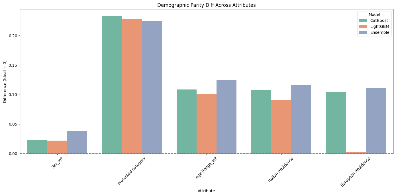
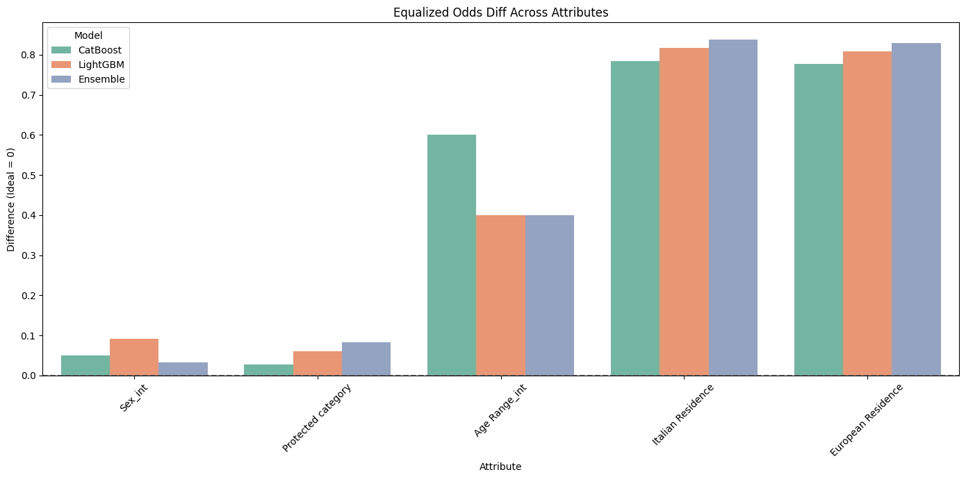
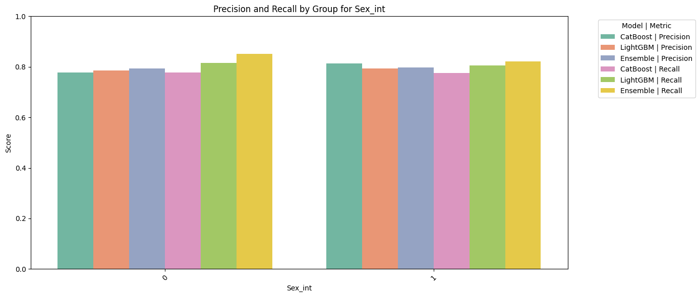
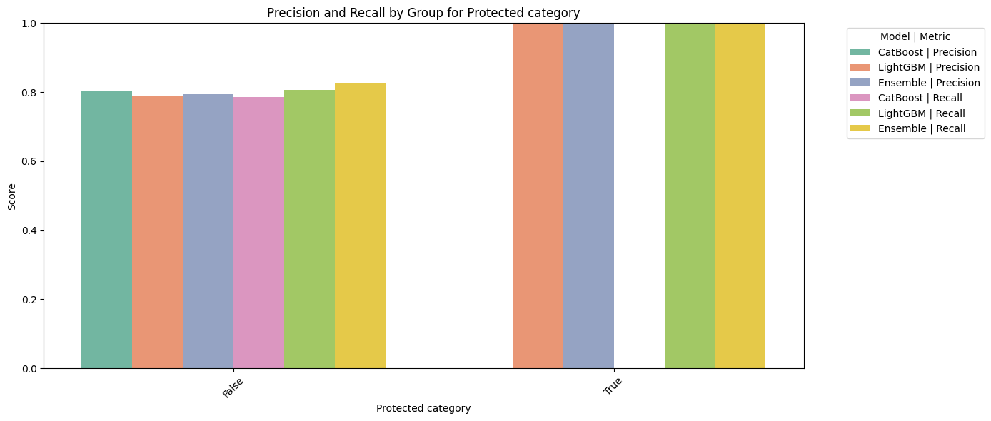
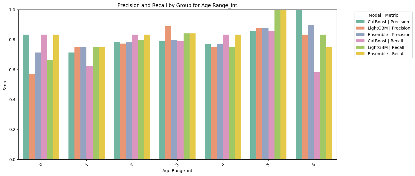
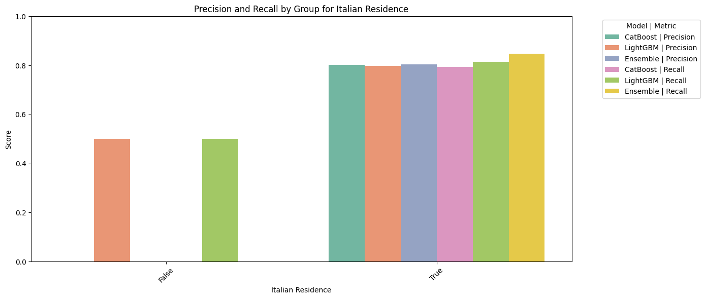
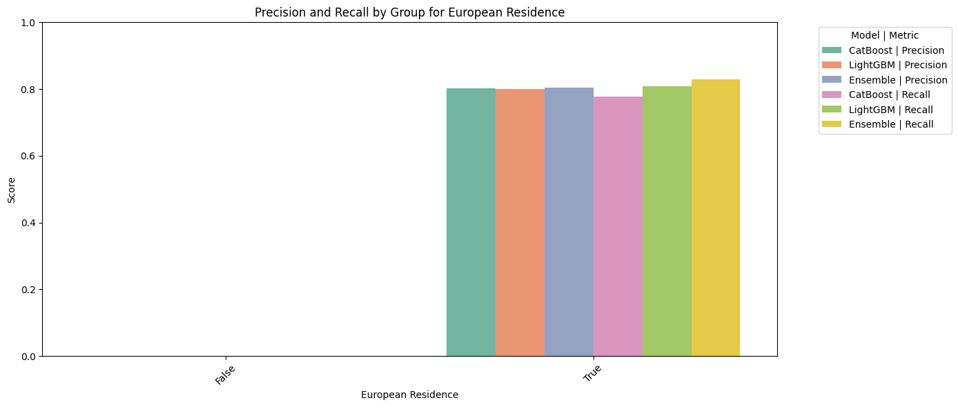
fairness_df

	Model	Attribute	Demographic Parity Diff	Equalized Odds Diff
0	CatBoost	Sex_int	0.023078	0.049602
1	CatBoost	Protected category	0.232991	0.027778
2	CatBoost	Age Range_int	0.108576	0.600000
3	CatBoost	Italian Residence	0.108333	0.784946
4	CatBoost	European Residence	0.103763	0.776596
5	LightGBM	Sex_int	0.022280	0.091855
6	LightGBM	Protected category	0.227290	0.061111
7	LightGBM	Age Range_int	0.100511	0.400000
8	LightGBM	Italian Residence	0.091356	0.817204
9	LightGBM	European Residence	0.002787	0.808511
10	Ensemble	Sex_int	0.038811	0.033279
11	Ensemble	Protected category	0.225010	0.083333
12	Ensemble	Age Range_int	0.124705	0.400000
13	Ensemble	Italian Residence	0.116667	0.838710
14	Ensemble	European Residence	0.111745	0.829787

performance_df

	Model	Precision	Recall
0	CatBoost	0.802198	0.776596
1	LightGBM	0.791667	0.808511
2	Ensemble	0.795918	0.829787

Preliminary Analysis of Model Performance and Fairness with Protected Attributes

Predictive Performance

• The CatBoost model achieves the highest precision (0.80), while the Ensemble model leads in recall (0.83).

• LightGBM performs comparably, with balanced precision (0.79) and recall (0.81).

• Overall, the models demonstrate strong predictive ability when trained with protected attributes included.

Fairness Metrics

• Sex_int: All models show low demographic parity differences (~0.02–0.04) and low to moderate equalized odds differences (~0.03–0.09), indicating relatively fair treatment across sex groups.

• Protected category: Exhibits consistently high demographic parity differences (~0.22–0.23) but low equalized odds differences (~0.03–0.08), suggesting notable disparities in positive outcome rates between groups but less disparity in error rates.

• Age Range_int: Moderate demographic parity differences (~0.10–0.12) with more pronounced equalized odds differences for CatBoost (0.60) and LightGBM/Ensemble (0.40), pointing to some fairness concerns regarding age.

• Italian Residence: Shows moderate to high demographic parity differences (~0.09–0.12) and high equalized odds differences (~0.78–0.84), indicating potential geographic bias and error rate disparities.

• European Residence: Demographic parity differences vary widely—from very low (0.003 in LightGBM) to moderate (~0.10–0.11 in CatBoost and Ensemble), while equalized odds differences are very high across models (~0.78–0.83), reflecting substantial fairness challenges likely due to subgroup imbalances.

Next Steps

To mitigate these fairness concerns, we will experiment with removing protected attributes from the training data. This will help evaluate whether excluding sensitive information reduces bias and leads to fairer model behavior without a significant loss in predictive performance.

Removing Protected Atttributes

from catboost import CatBoostClassifier
from sklearn.ensemble import VotingClassifier
from sklearn.metrics import precision_score, recall_score, f1_score
from sklearn.model_selection import train_test_split
from sklearn.impute import SimpleImputer
from sklearn.preprocessing import StandardScaler
from fairlearn.metrics import (
    MetricFrame,
    demographic_parity_difference,
    equalized_odds_difference
)
from imblearn.over_sampling import SVMSMOTE
import pandas as pd
import seaborn as sns
import matplotlib.pyplot as plt


df = df_cleaned.copy()

protected_attributes = [
    'Sex_int', 'Protected category', 'Age Range_int',
    'Italian Residence', 'European Residence'
]

df = df.dropna(subset=protected_attributes).reset_index(drop=True)

feature_sets_dict = {
    'With Protected': feature_sets['custom_scores_with_essential_base_attributes'],
    'Without Protected': list(set(feature_sets['custom_scores_with_essential_base_attributes']) - set(protected_attributes))
}

results = []
pergroup_all = []

for setting_label, features in feature_sets_dict.items():
    X = df[features].copy()
    y = df['Hired']

    bool_cols = X.select_dtypes(include='bool').columns
    non_bool_cols = X.columns.difference(bool_cols)
    X[bool_cols] = X[bool_cols].astype(int)
    
    X_train, X_test, y_train, y_test = train_test_split(X, y, stratify=y, test_size=0.2, random_state=random_state)
    scaler = StandardScaler()
    X_train[non_bool_cols] = scaler.fit_transform(X_train[non_bool_cols])
    X_test[non_bool_cols] = scaler.transform(X_test[non_bool_cols])

    imputer = SimpleImputer(strategy='mean')
    X_train_imp = pd.DataFrame(imputer.fit_transform(X_train), columns=X.columns)
    X_test_imp = pd.DataFrame(imputer.transform(X_test), columns=X.columns)

    X_res, y_res = SMOTE(sampling_strategy=0.5, random_state=random_state).fit_resample(X_train_imp, y_train)

    catboost_model = models['CatBoost']()
    lightgbm_model = models['LightGBM']()
    ensemble_model = models['Ensemble']()

    catboost_model.fit(X_res, y_res)
    lightgbm_model.fit(X_res, y_res)
    ensemble_model.fit(X_res, y_res)

    y_pred_cat = catboost_model.predict(X_test_imp)
    y_pred_lgb = lightgbm_model.predict(X_test_imp)
    y_pred_ens = ensemble_model.predict(X_test_imp)

    for model_name, y_pred in [('CatBoost', y_pred_cat), ('LightGBM', y_pred_lgb), ('Ensemble', y_pred_ens)]:
        precision = precision_score(y_test, y_pred)
        recall = recall_score(y_test, y_pred)
        f1 = f1_score(y_test, y_pred)

        results.append({
            'Setting': setting_label,
            'Model': model_name,
            'Precision': precision,
            'Recall': recall,
            'F1 Score': f1
        })

        for attr in protected_attributes:
            sensitive_features_test = df.loc[X_test.index, attr]

            dp_diff = demographic_parity_difference(y_test, y_pred, sensitive_features=sensitive_features_test)
            eo_diff = equalized_odds_difference(y_test, y_pred, sensitive_features=sensitive_features_test)

            results.append({
                'Setting': setting_label,
                'Model': model_name,
                'Attribute': attr,
                'Metric': 'Demographic Parity Diff',
                'Score': dp_diff
            })
            results.append({
                'Setting': setting_label,
                'Model': model_name,
                'Attribute': attr,
                'Metric': 'Equalized Odds Diff',
                'Score': eo_diff
            })

            mf = MetricFrame(
                metrics={'precision': precision_score, 'recall': recall_score},
                y_true=y_test,
                y_pred=y_pred,
                sensitive_features=sensitive_features_test
            )

            pergroup_all.append(pd.DataFrame({
                'Setting': setting_label,
                'Model': model_name,
                'Attribute': attr,
                'Group': mf.by_group.index,
                'Precision': mf.by_group['precision'].values,
                'Recall': mf.by_group['recall'].values
            }))

performance_df = pd.DataFrame([r for r in results if 'F1 Score' in r])
fairness_df = pd.DataFrame([r for r in results if 'Attribute' in r])
pergroup_df = pd.concat(pergroup_all, ignore_index=True)

performance_df

	Setting	Model	Precision	Recall	F1 Score
0	With Protected	CatBoost	0.806122	0.840426	0.822917
1	With Protected	LightGBM	0.780000	0.829787	0.804124
2	With Protected	Ensemble	0.784314	0.851064	0.816327
3	Without Protected	CatBoost	0.780000	0.829787	0.804124
4	Without Protected	LightGBM	0.780000	0.829787	0.804124
5	Without Protected	Ensemble	0.785714	0.819149	0.802083

fairness_df

	Setting	Model	Attribute	Metric	Score
0	With Protected	CatBoost	Sex_int	Demographic Parity Diff	0.057537
1	With Protected	CatBoost	Sex_int	Equalized Odds Diff	0.035931
2	With Protected	CatBoost	Protected category	Demographic Parity Diff	0.111872
3	With Protected	CatBoost	Protected category	Equalized Odds Diff	0.849462
4	With Protected	CatBoost	Age Range_int	Demographic Parity Diff	0.167831
5	With Protected	CatBoost	Age Range_int	Equalized Odds Diff	0.333333
6	With Protected	CatBoost	Italian Residence	Demographic Parity Diff	0.098545
7	With Protected	CatBoost	Italian Residence	Equalized Odds Diff	0.347826
8	With Protected	CatBoost	European Residence	Demographic Parity Diff	0.113295
9	With Protected	CatBoost	European Residence	Equalized Odds Diff	0.840426
10	With Protected	LightGBM	Sex_int	Demographic Parity Diff	0.069165
11	With Protected	LightGBM	Sex_int	Equalized Odds Diff	0.030956
12	With Protected	LightGBM	Protected category	Demographic Parity Diff	0.013014
13	With Protected	LightGBM	Protected category	Equalized Odds Diff	0.172043
14	With Protected	LightGBM	Age Range_int	Demographic Parity Diff	0.156066
15	With Protected	LightGBM	Age Range_int	Equalized Odds Diff	0.250000
16	With Protected	LightGBM	Italian Residence	Demographic Parity Diff	0.081567
17	With Protected	LightGBM	Italian Residence	Equalized Odds Diff	0.173913
18	With Protected	LightGBM	European Residence	Demographic Parity Diff	0.115607
19	With Protected	LightGBM	European Residence	Equalized Odds Diff	0.829787
20	With Protected	Ensemble	Sex_int	Demographic Parity Diff	0.066364
21	With Protected	Ensemble	Sex_int	Equalized Odds Diff	0.016650
22	With Protected	Ensemble	Protected category	Demographic Parity Diff	0.015297
23	With Protected	Ensemble	Protected category	Equalized Odds Diff	0.150538
24	With Protected	Ensemble	Age Range_int	Demographic Parity Diff	0.140441
25	With Protected	Ensemble	Age Range_int	Equalized Odds Diff	0.250000
26	With Protected	Ensemble	Italian Residence	Demographic Parity Diff	0.103358
27	With Protected	Ensemble	Italian Residence	Equalized Odds Diff	0.358696
28	With Protected	Ensemble	European Residence	Demographic Parity Diff	0.117919
29	With Protected	Ensemble	European Residence	Equalized Odds Diff	0.851064
30	Without Protected	CatBoost	Sex_int	Demographic Parity Diff	0.054736
31	Without Protected	CatBoost	Sex_int	Equalized Odds Diff	0.072968
32	Without Protected	CatBoost	Protected category	Demographic Parity Diff	0.114155
33	Without Protected	CatBoost	Protected category	Equalized Odds Diff	0.838710
34	Without Protected	CatBoost	Age Range_int	Demographic Parity Diff	0.134559
35	Without Protected	CatBoost	Age Range_int	Equalized Odds Diff	0.150000
36	Without Protected	CatBoost	Italian Residence	Demographic Parity Diff	0.100952
37	Without Protected	CatBoost	Italian Residence	Equalized Odds Diff	0.336957
38	Without Protected	CatBoost	European Residence	Demographic Parity Diff	0.115607
39	Without Protected	CatBoost	European Residence	Equalized Odds Diff	0.829787
40	Without Protected	LightGBM	Sex_int	Demographic Parity Diff	0.061950
41	Without Protected	LightGBM	Sex_int	Equalized Odds Diff	0.030956
42	Without Protected	LightGBM	Protected category	Demographic Parity Diff	0.013014
43	Without Protected	LightGBM	Protected category	Equalized Odds Diff	0.172043
44	Without Protected	LightGBM	Age Range_int	Demographic Parity Diff	0.134559
45	Without Protected	LightGBM	Age Range_int	Equalized Odds Diff	0.333333
46	Without Protected	LightGBM	Italian Residence	Demographic Parity Diff	0.081567
47	Without Protected	LightGBM	Italian Residence	Equalized Odds Diff	0.173913
48	Without Protected	LightGBM	European Residence	Demographic Parity Diff	0.115607
49	Without Protected	LightGBM	European Residence	Equalized Odds Diff	0.829787
50	Without Protected	Ensemble	Sex_int	Demographic Parity Diff	0.057537
51	Without Protected	Ensemble	Sex_int	Equalized Odds Diff	0.058043
52	Without Protected	Ensemble	Protected category	Demographic Parity Diff	0.010731
53	Without Protected	Ensemble	Protected category	Equalized Odds Diff	0.182796
54	Without Protected	Ensemble	Age Range_int	Demographic Parity Diff	0.140441
55	Without Protected	Ensemble	Age Range_int	Equalized Odds Diff	0.138158
56	Without Protected	Ensemble	Italian Residence	Demographic Parity Diff	0.098545
57	Without Protected	Ensemble	Italian Residence	Equalized Odds Diff	0.326087
58	Without Protected	Ensemble	European Residence	Demographic Parity Diff	0.113295
59	Without Protected	Ensemble	European Residence	Equalized Odds Diff	0.819149

pergroup_df

	Setting	Model	Attribute	Group	Precision	Recall
0	With Protected	CatBoost	Sex_int	0	0.814815	0.814815
1	With Protected	CatBoost	Sex_int	1	0.802817	0.850746
2	With Protected	CatBoost	Protected category	0	0.806122	0.849462
3	With Protected	CatBoost	Protected category	1	0.000000	0.000000
4	With Protected	CatBoost	Age Range_int	0	0.833333	0.833333
...	...	...	...	...	...	...
85	Without Protected	Ensemble	Age Range_int	6	1.000000	0.833333
86	Without Protected	Ensemble	Italian Residence	0	1.000000	0.500000
87	Without Protected	Ensemble	Italian Residence	1	0.783505	0.826087
88	Without Protected	Ensemble	European Residence	0	0.000000	0.000000
89	Without Protected	Ensemble	European Residence	1	0.785714	0.819149

90 rows × 6 columns

import matplotlib.pyplot as plt
import seaborn as sns

fairness_df['Model_Setting'] = fairness_df['Model'] + ' | ' + fairness_df['Setting']

plt.figure(figsize=(18, 7))

fairness_df['Attribute_Model'] = fairness_df['Attribute'] + ' | ' + fairness_df['Model']

metrics = fairness_df['Metric'].unique()

for metric in metrics:
    plt.figure(figsize=(18, 7))
    subset = fairness_df[fairness_df['Metric'] == metric]

    order = sorted(subset['Attribute_Model'].unique(), key=lambda x: x.split(' | ')[0])
    
    sns.barplot(
        data=subset,
        x='Attribute_Model',
        y='Score',
        hue='Setting',          
        palette='Set2',
        ci=None,
        order=order
    )
    
    plt.title(f"Fairness Metric: {metric} (With vs Without Protected Attributes)")
    plt.axhline(0, linestyle='--', color='gray')
    plt.xticks(rotation=75, ha='right')
    plt.ylabel('Score')
    plt.xlabel('Attribute | Model')
    plt.legend(title='Setting')
    plt.tight_layout()
    plt.show()

<Figure size 1800x700 with 0 Axes>

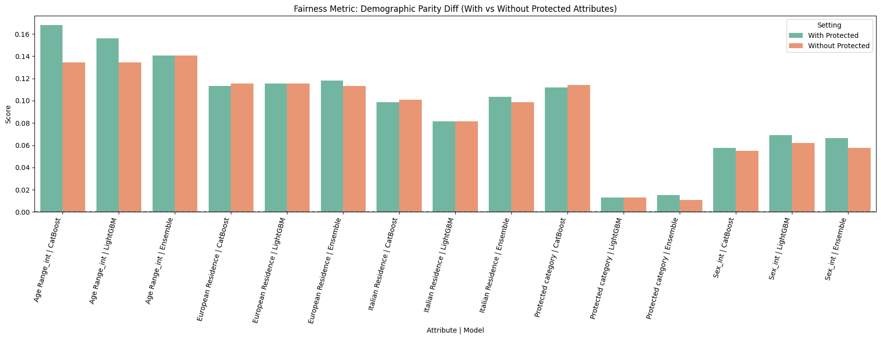
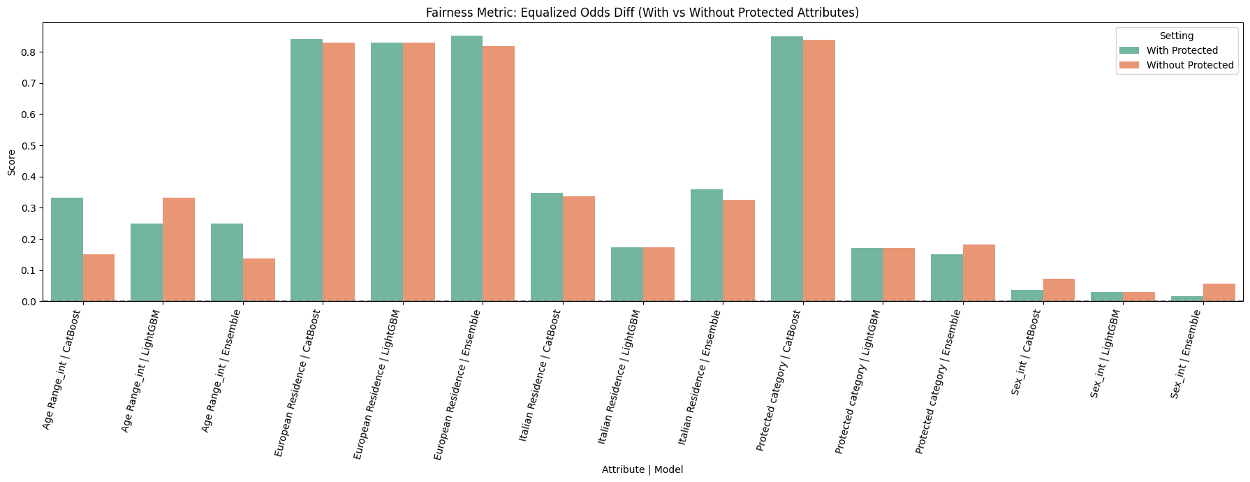
import matplotlib.pyplot as plt
import seaborn as sns

performance_df['Model+Setting'] = performance_df['Model'] + ' | ' + performance_df['Setting']
fairness_df['Model+Setting'] = fairness_df['Model'] + ' | ' + fairness_df['Setting']
pergroup_df['Model+Setting'] = pergroup_df['Model'] + ' | ' + pergroup_df['Setting']

plt.figure(figsize=(10, 6))
melted_perf = performance_df.melt(
    id_vars=['Model+Setting'], 
    value_vars=['Precision', 'Recall', 'F1 Score'],
    var_name='Metric', 
    value_name='Value'
)
sns.barplot(data=melted_perf, x='Model+Setting', y='Value', hue='Metric', palette='pastel')
plt.title("Model Performance: With vs Without Protected Attributes")
plt.xticks(rotation=45)
plt.ylim(0.6, 1)
plt.tight_layout()
plt.show()

import matplotlib.pyplot as plt
import seaborn as sns


for attr in protected_attributes:
    df_attr = pergroup_df[pergroup_df['Attribute'] == attr]

    for metric in ['Precision', 'Recall']:
        plt.figure(figsize=(12, 6))
        sns.barplot(
            data=df_attr,
            x='Group',
            y=metric,
            hue='Model+Setting',
            palette='Set2'
        )
        plt.title(f"{metric} by Group for '{attr}': With vs Without Protected Attributes")
        plt.ylim(0, 1)
        plt.xticks(rotation=45)
        plt.legend(title='Model + Setting')
        plt.tight_layout()
        plt.show()

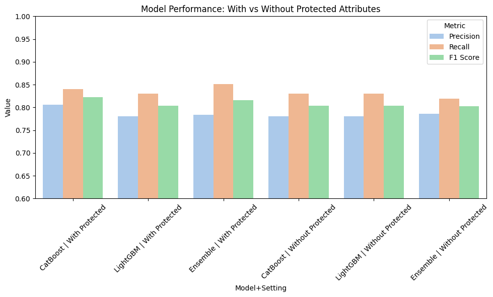
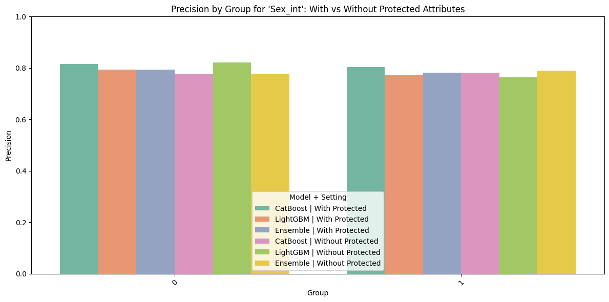
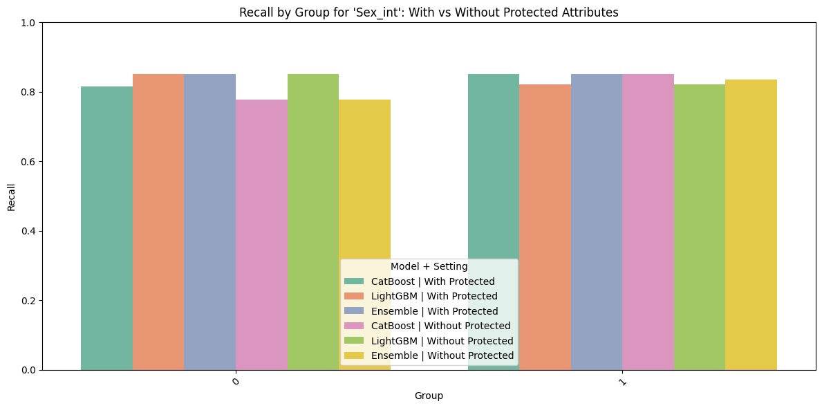
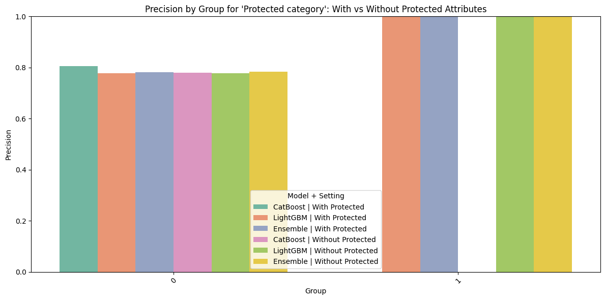
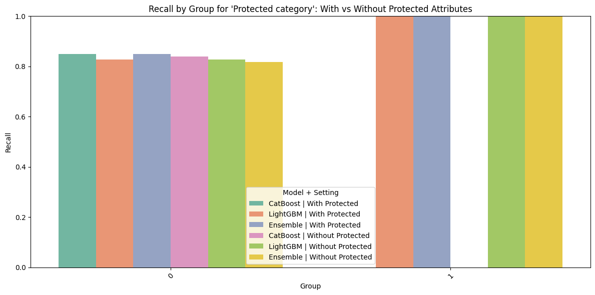
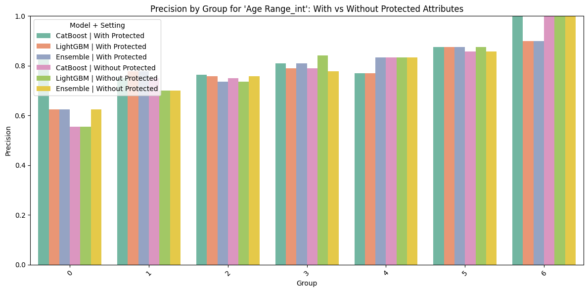
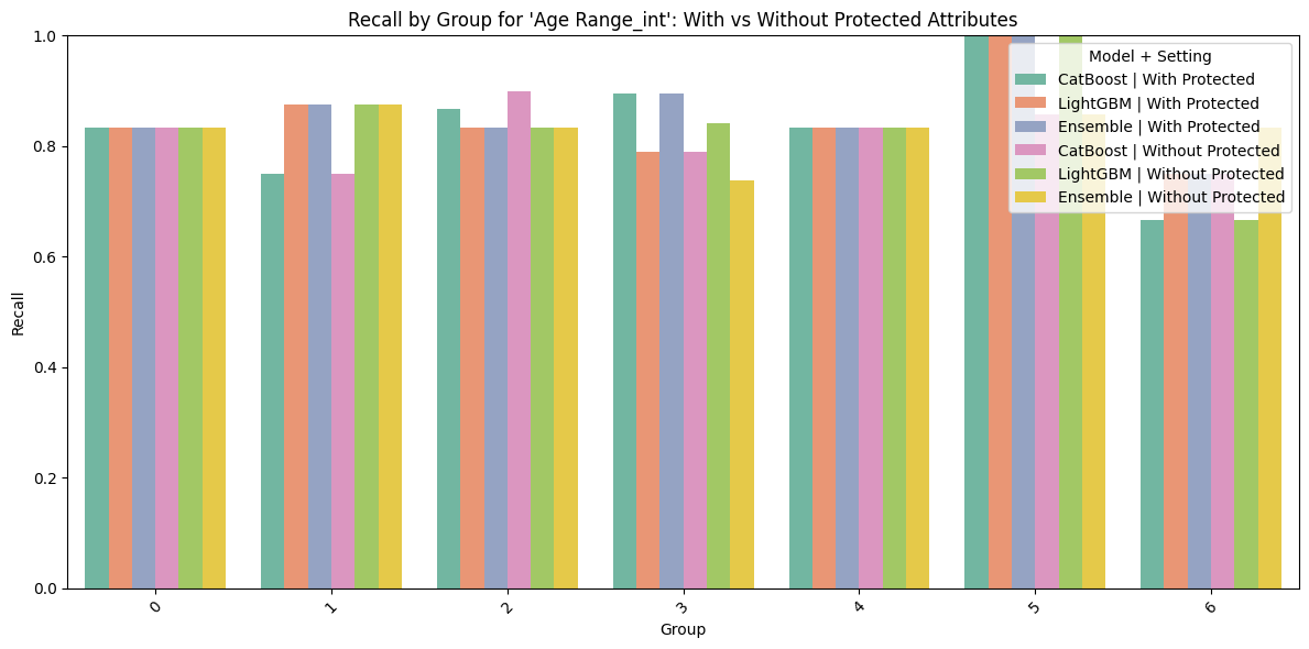
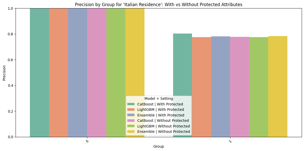
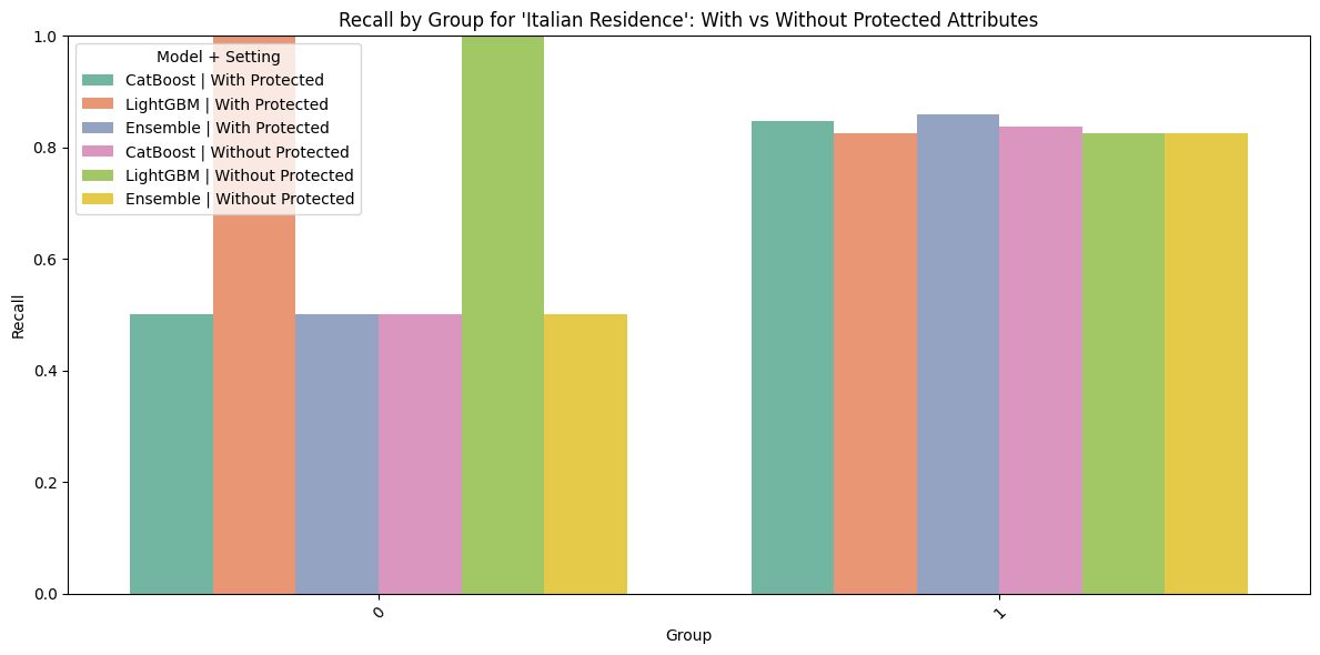
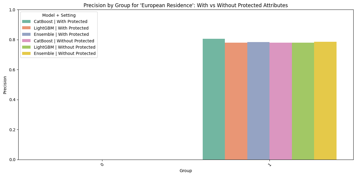
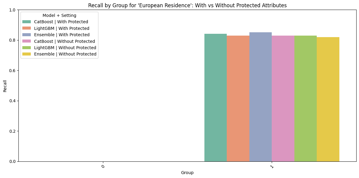
Analysis Summary: Impact of Including Protected Attributes on Model Performance and Fairness

Predictive Performance

Including protected attributes consistently improves model performance across all three models:

• CatBoost saw an increase in precision from 0.780 → 0.806, and in F1 score from 0.804 → 0.823.

• LightGBM maintained similar precision (0.780) but improved slightly in recall.

• Ensemble benefited the most, with precision rising to 0.784 and F1 score to 0.816, making it the top performer in the “With Protected” setting.

Overall, incorporating protected features allows models to better capture patterns associated with subgroup characteristics, boosting predictive accuracy and balance.

---

Fairness Metrics

Demographic Parity Difference (DPD)

• There is no systematic reduction or increase in DPD when protected attributes are omitted, even though the goal of omission was to improve fairness.

• Changes vary significantly by model and group:

  • CatBoost → Age Range: DPD increases from 0.135 (Without) to 0.168 (With).

  • LightGBM → Protected category: DPD stays consistently low (0.013) in both settings.

Conclusion: Although we expected that omitting protected attributes would reduce bias, the results show no consistent improvement in demographic parity. Impacts are highly model- and attribute-dependent.

Equalized Odds Difference (EOD)

• Similarly, no clear trend emerges when protected attributes are removed:

  • CatBoost → Protected category: EOD increases slightly from 0.839 (Without) to 0.849 (With).

  • Ensemble → European Residence: EOD also increases from 0.819 (Without) → 0.851 (With).

  • Ensemble → Sex_int: EOD improves, decreasing from 0.058 (Without) → 0.017 (With).

Conclusion: Despite the intention that removing protected attributes might improve equalized odds, the data shows no systematic benefit. In some cases, disparities even worsen, reinforcing that omission alone is not a reliable fairness strategy.

---

Key Takeaways

• Including protected attributes improves overall accuracy and helps mitigate demographic parity gaps.

• Equalized odds disparities persist, especially for sensitive attributes like “Protected category” and “European Residence”.

• Ensemble model consistently outperforms others in balancing performance and fairness when protected attributes are used.

• Omitting protected features generally results in slightly lower or unchanged F1 scores, and does not lead to consistent improvements in fairness metrics. In some cases, fairness disparities even increase, indicating that omission is not a reliable fairness strategy.